Hello reader, welcome to my Know The Math series, a less formal series of blogs, where I take you through the notoriously complex backend mathematics which forms the soul for machine learning algorithms. I try and summarise works of famous researchers, put them as my notes and share with everyone in hopes that it might be helpful for you too!
Before we begin, I need you to conduct a ceremony:
- Stand up in front of a mirror, and say it out aloud, “I am going to learn the Math behind HMM & the Forward Algorithm, today!”
- Take a out a naice register & pen to go through the derivation with me.
Contents
- Introduction
- The components of Hidden Markov Model
- First-Order HMM & its Assumptions
- 3 Fundamental problems of HMM
- Understanding the Case & Example
- The Forward Algorithm
- References
Introduction
A Hidden Markov Model helps us operate on probability distribution on a given sequence (more often a times-series) where the sequence is assumed to be a Markov process. This mini-blog aims to explore this, and it’s more like my personal note on the concept which I am sharing with all. I’ve learnt almost entirity of the concept from the great Professor Daniel Jurafsky and will be borrowing the content from his works available on the net. I’ll try and summarise his work given over here, as quick notes!
The components of Hidden Markov Model
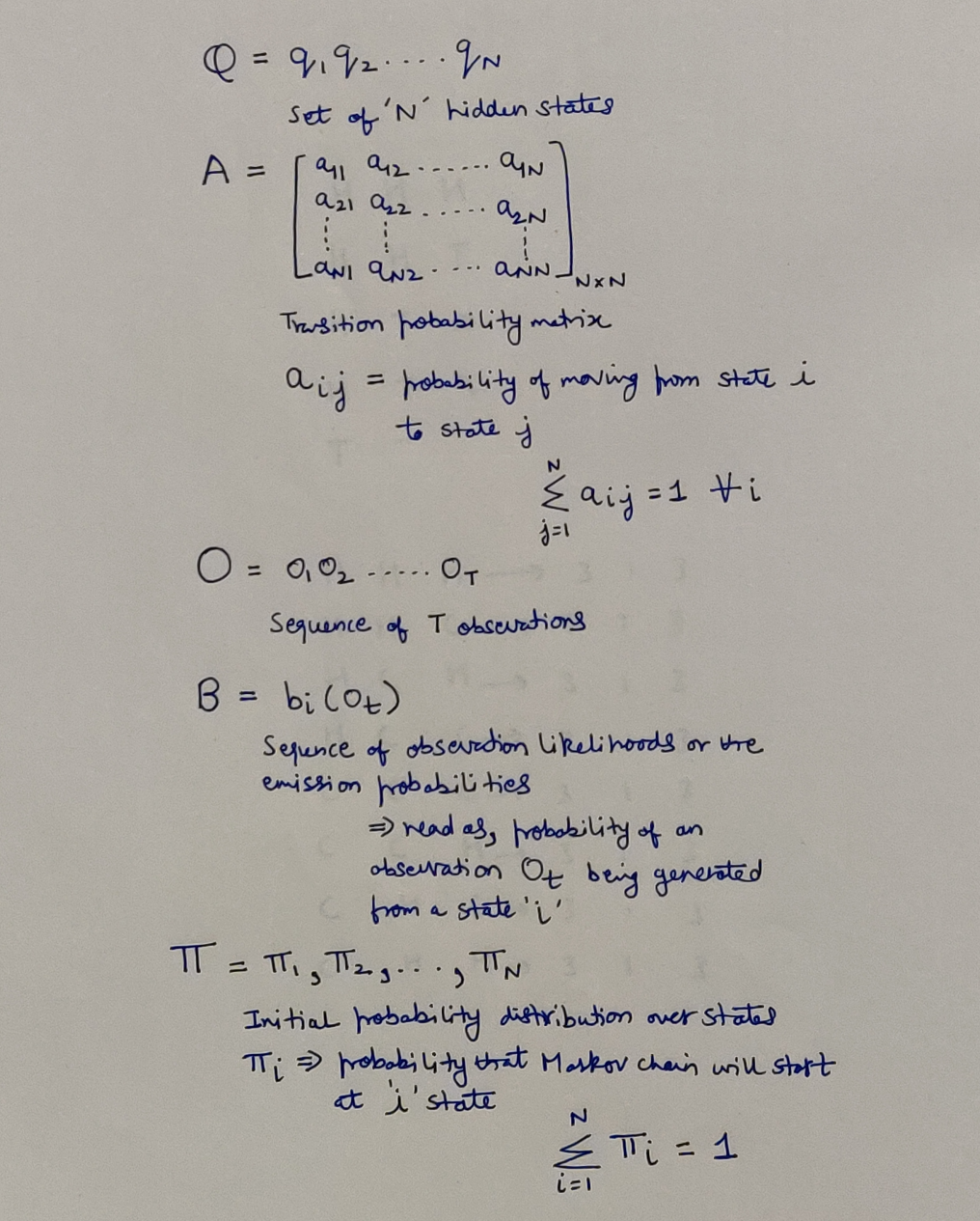 HMM Components, source: Jurafsky’s work
First-Order HMM & its Assumptions
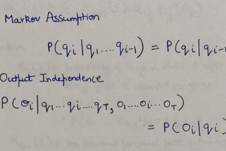
- Markov Assumption: The probability of particular state depends only on previous state.
- Output Independence: The probability of a particular observation O_i depends only on the state that produced the observation q_i & not on any other states or any other observations.
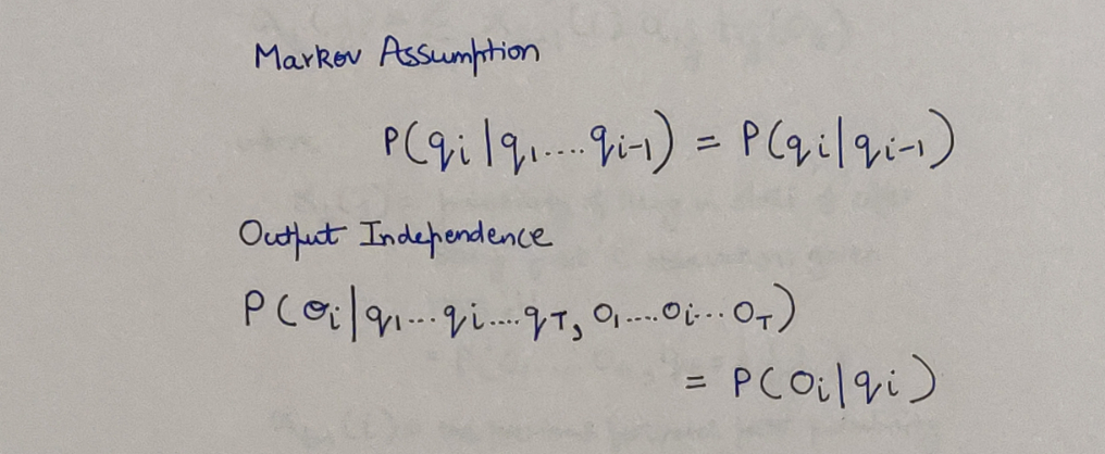 First Order HMM & its assumptions, source: Jurafsky’s work
3 Fundamental problems of HMM
The HMM helps us deal with 3 fundamental problems. Each has its unique ways to go about it.
- Problem 1 - Likelihood - Given an HMM λ = (A,B) and an observation sequence O, determine the likelihood P(O|λ).
- Problem 2 - Decoding - Given an observation sequence O and an HMM λ = (A,B), discover the best hidden state sequence Q.
- Problem 3 - Learning - Given an observation sequence O and the set of states in the HMM, learn the HMM parameters A and B.
Understanding the Case & Example
Jurafsky’s work employs Jason Eisner’s work, and uses the following example to build and explain the above-mentioned problems.
Let’s say that you are a climatologist from a distant future and are interested in weather in Baltimore, Maryland, for the summer of 2020. What you don’t have is the weather record from this time, but what you do have is Eisner’s diary from that time which details as to how many ice-creams Eisner had every day during that summer. So here, the number of ice-creams Eisner had everyday is the sequence of observations that we witness, and the temperature on every corresponding day which have no clue of (i.e. hidden to us) is the sequence of hidden states which influence Eisner for the number of ice creams he eats. For simplicity, we’ll have only 2 type of days - Hot or Cold, and Eisner can have maximum of 3 and minimum of 1 ice-cream on any given day. Naturally, one can understand that on Hot days Eisner is more probable to eat ice creams and opposite for Cold days.
- Q = {H, C} # The Hidden States
- V = {1,2,3} # The vocabulary or The alphabet from which an observation sequence can be generated
Understanding the given case, source: Jurafsky’s work
The Forward Algorithm
This algorithm will help us solve the first problem as mentioned above. From the example, we can informally state the problem as let’s say, What is the probability of observing the sequence -: 3 - 1 - 3 ? What is the probability that Eisner eats 3 ice creams the 1st day, 1 ice cream the 2nd day and 3 ice creams the 3rd day? Now, what about the underlying hidden states? Each of those days, it can either be Cold or Hot, and since there are 2 possible days in sequence, we have 8 (2^3) possibilites/permutation of the hidden states.
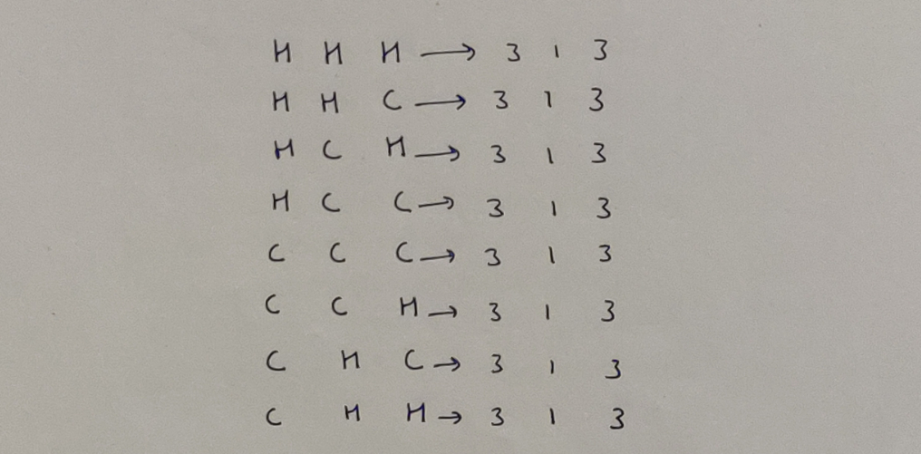 The possible hidden state combinations that can result in our observed sequence of 3-1-3
For HMM with N hidden states and an observation sequence of length T, there are N^T possible hidden sequences.
So to find out the likelihood of the given observation sequence, we have the Forward Algorithm which has a worst case time complexity of O(TN^2) optimised by Dynamic Programming. We are going to generate all possible sequences and take sum over their probabilities to arrive at our desired likelihood.
Seeing how we explore all hidden sequences and find out all probabilties, source: Jurafsky’s work
In the algorithm, probability at every hidden state has been simplified as alpha functions.
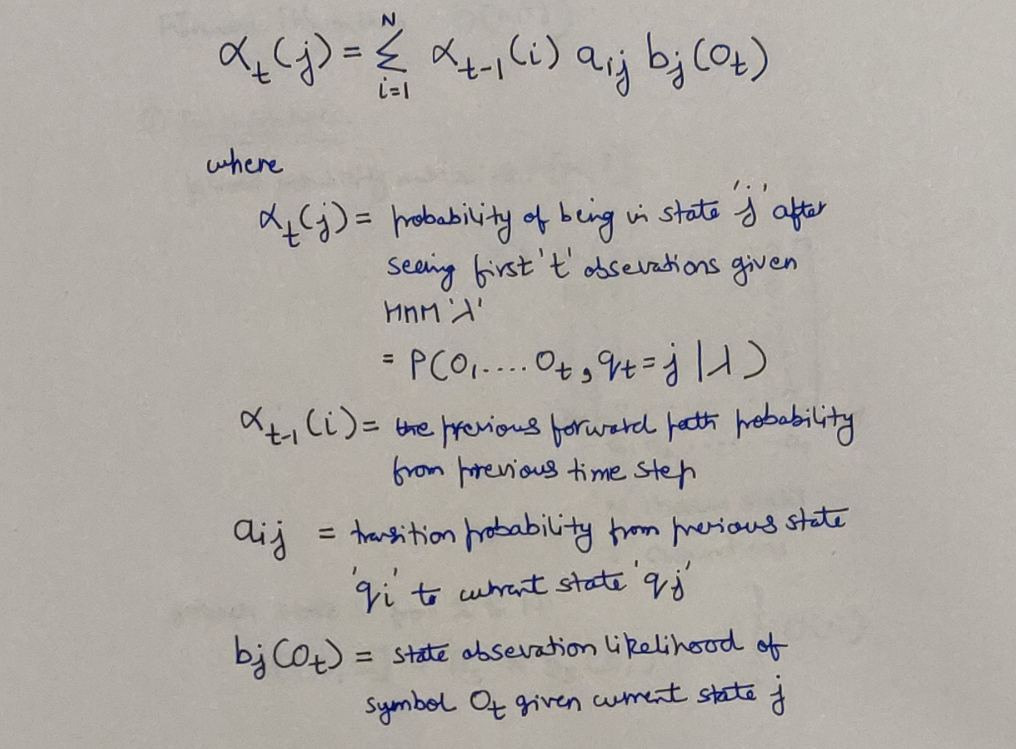 The Alpha function, source: Jurafsky’s work
The algorithm in whole, can be generalised as:
Generalising the computations, source: Jurafsky’s work
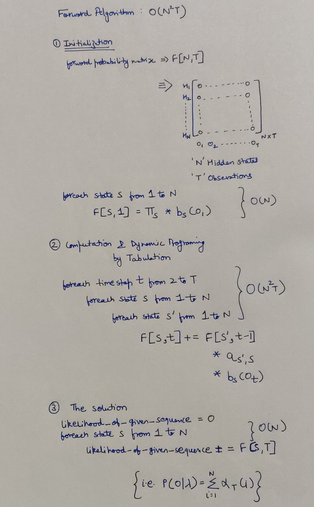 Algorithm Pseudocode & Time Series Analysis
Hope I was able to help you out with the concepts mentioned! I would also request to have a look at the original work, since this is just a summarised version of it for quick revision. Thank you so much Professor Jurafsky for the pathbreaking work.
I’ll be continuing the HMM series, we’ll talk about the Problem 2 next & the Viterbi Algorithm to solve it!
References
- https://web.stanford.edu/~jurafsky/slp3/A.pdf
- https://cs.jhu.edu/~jason/papers/eisner.tnlp02.pdf
- http://mlg.eng.cam.ac.uk/zoubin/papers/ijprai.pdf
- https://towardsdatascience.com/introduction-to-hidden-markov-models-cd2c93e6b781
यस्त्वात्मरतिरेव स्यादात्मतृप्तश्च मानवः ।
आत्मन्येव च सन्तुष्टस्तस्य कार्यं न विद्यते ॥
– Bhagavad Gita 3.17 ॥
(Read about this Shloka from the Bhagavad Gita here at http://sanskritslokas.com/)
 Know The Math - The Principal Component Analysis algorithm