Hello reader, welcome to my Know The Math series, a less formal series of blogs, where I take you through the notoriously complex backend mathematics which forms the soul for machine learning algorithms. The idea for the series originated from my Project - NIFTYBANK Index Time series analysis, Prediction, Deep Learning & Bayesian Hyperparameter Optimization where people also asked to explain the underlying concepts.
Before we begin, I need you to conduct a ceremony:
- Stand up in front of a mirror, and say it out aloud, “I am going to learn the Math behind Linear Regression modelling - getting the Intercept & Slope coefficients, today!”
- Take a out a naice register & pen to go through the derivation with me.
Contents
- Assumptions for Linear Regression
- Understanding the Given Equations
- A Simple Derivation
- Diving Deeper into the Math
- References
Assumptions for Linear Regression
Before we proceed with the derivation of our Linear Regression coefficients, let us first refresh our memory and list down the assumptions we make when we apply this algorithm. Allow me to borrow these lines from the CFA curriculum:
- A linear relationship exists between the dependent & the independent variable
- The independent variable is uncorrelated with the residuals
- The expected value of residual term is zero
- The variance of the residual term is constant for all observations
- The residual term is independently & normally distributed
Understanding the Given Equations
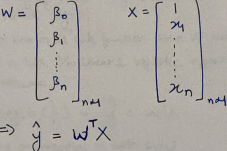
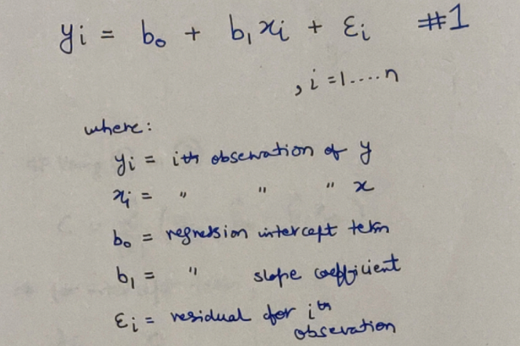
Let us for a given dataset assume, that the all-knowing Lord Vishnu (from the Hindu Mythology) comes and gives you the Linear Regression model. It looks somewhat like this:
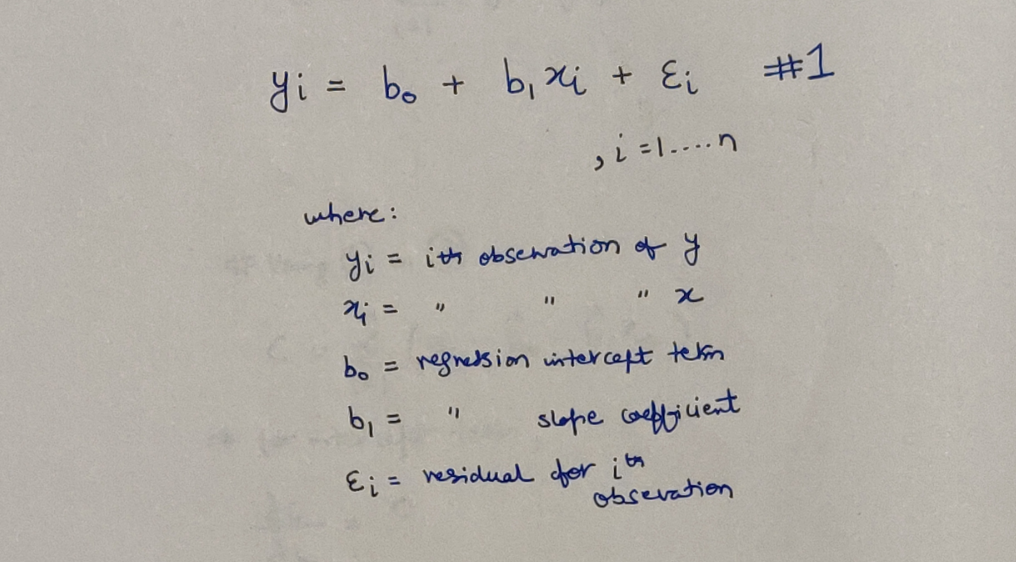 The perfect Linear Regression Model
And, you an earthling, are going to prepare a Linear Regression model from the same dataset in hopes that it is very close to the above one. Our model is somewhat going to look like this:
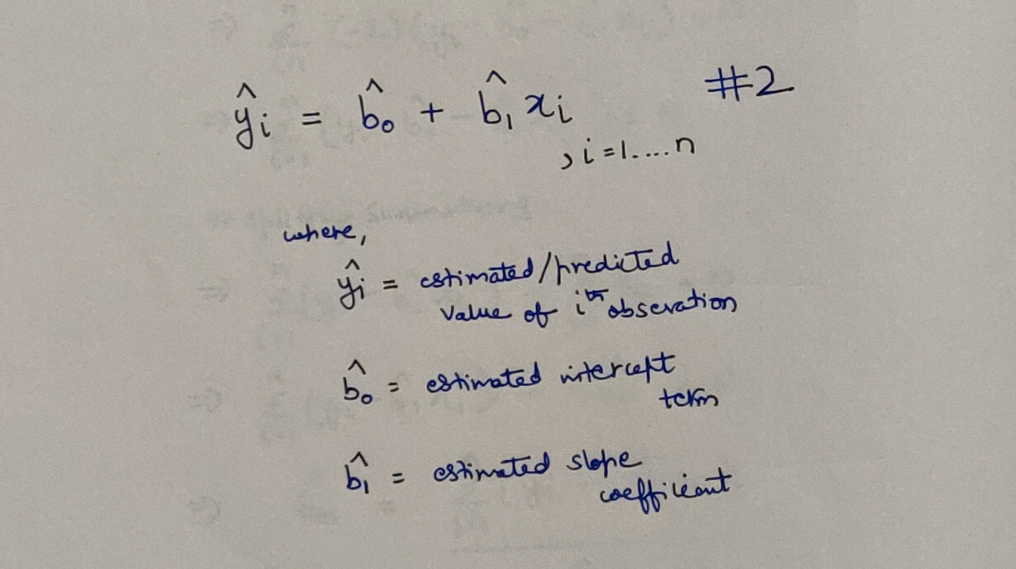 Our attempt at Linear Regression Model
Now, the question is, how do I get those values of the Intercept & Slope coefficients? Let’s get started.
A Simple Derivation
We know, that our model will be the best, if we can minimize the difference between our predicted and the actual values of the dependent variable. Most commonly, the difference is formally represented as Sum of Squared Errors (SSE) where in each error is the difference between the predicted value and the actual value of the corresponding data point. We will call this expression, as our Cost Function. Here is how it looks like:
 The Cost Function
Borrowing from common wisdom, one can conclude, that lesser the value of this Cost Function, the better will be our Linear Regression model. And now, how I want you to look at it is as follows:
Forget all things, buzzwords & concepts like Machine Learning, Linear Regression, Prediction, Deep Learning and all earthly things for that matter. In this entire universe, there is only you and this Cost Function that you have to minimize. This essentially is only an optimization problem and give it only the respect that such a problem deserves. Don’t let anyone scare you and make you feel otherwise!
We find the minima (where our Cost Function is minimized) by using Derivatives, more specifically setting the partial derivatives equal to Zero.
Finding the Intercept Term
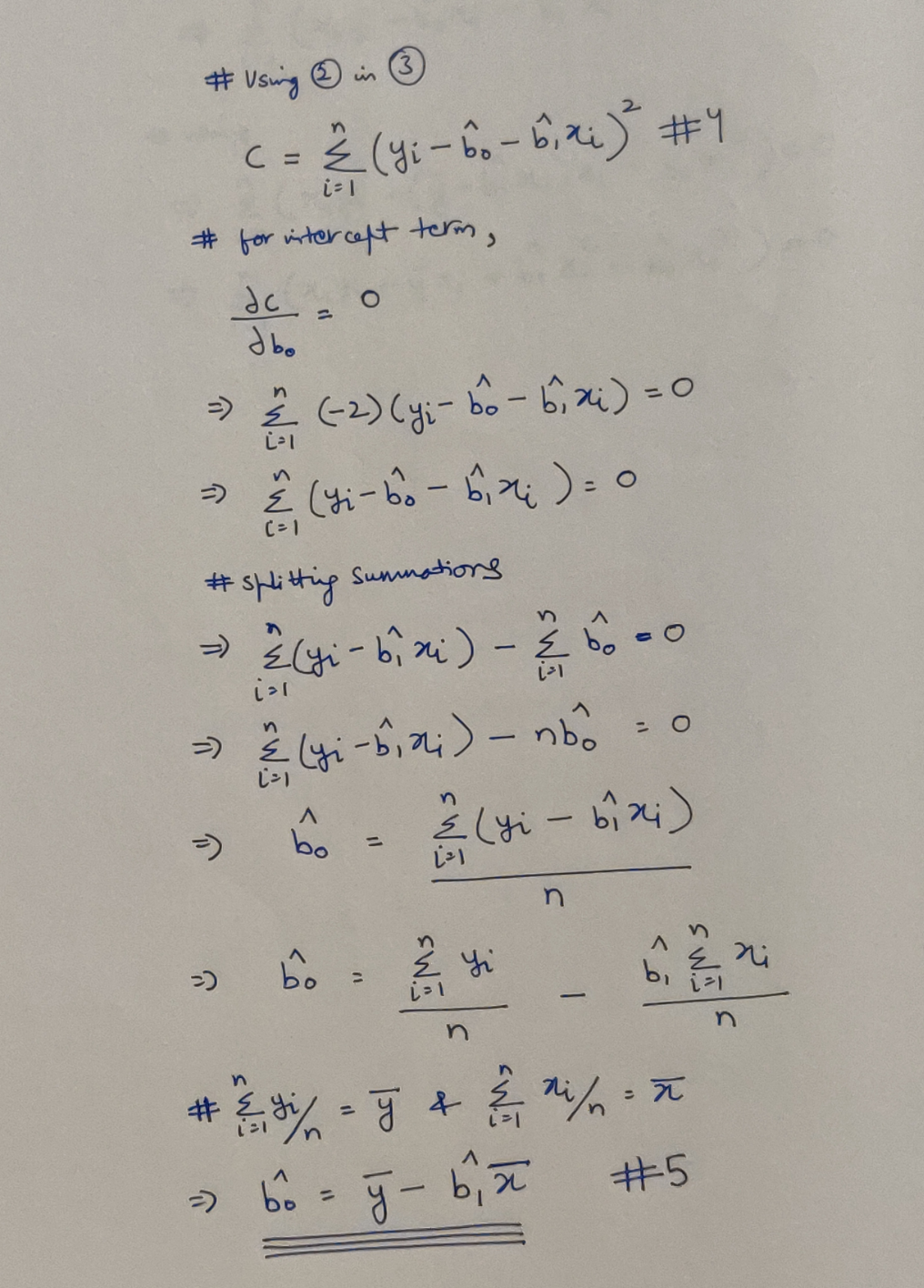 Finding our Intercept Term
Finding the Slope Coefficient
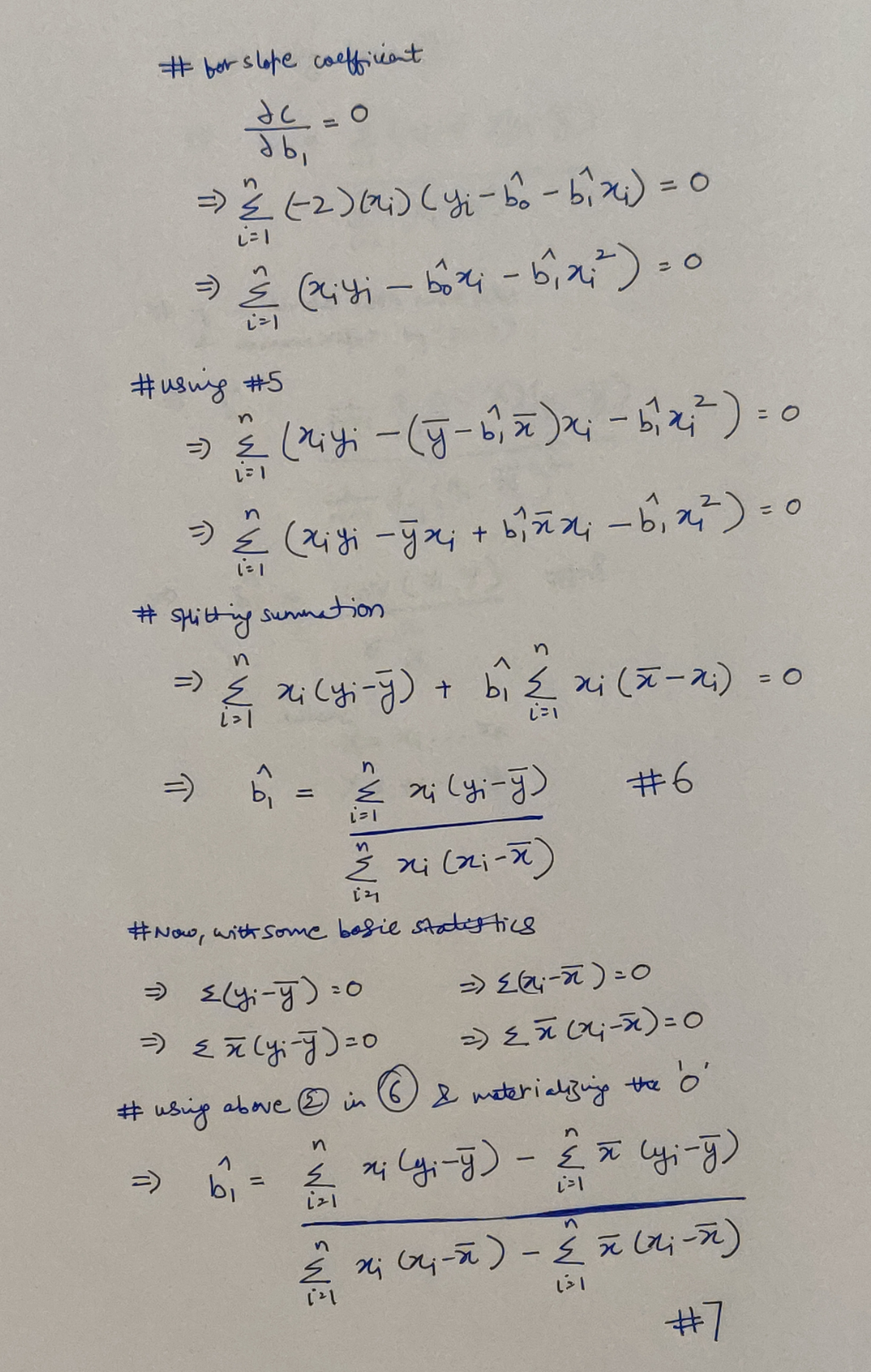 Finding our Slope Coefficient
We could have stopped at Equation 6, but as it happens, we can derive a more prominent variation! Here is how:
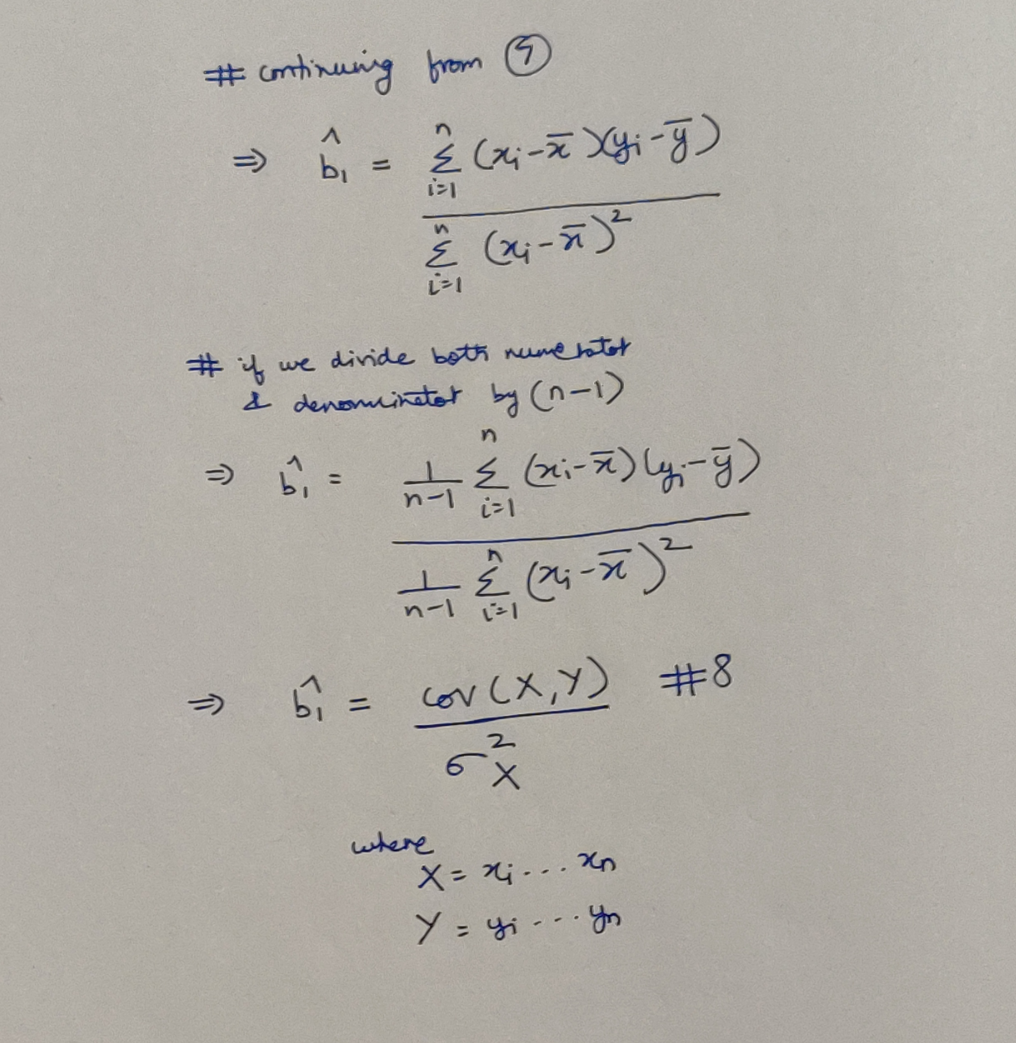 Reshaping our Slope Coefficient
Diving Deeper into the Math
Well, the issue is, setting the partial derivatives to zero, gives us the power to get an extrema (a minima or a maxima) and here lies the problem! We don’t know whether what we have found is a really a minima? Or a maxima? To know all this, we’ll have to investigate further. KEYWORDS: Jacobian(J) & Hessian(H). Again, don’t be scared, we just need to find more derivatives. And Jacobian? Well we already have that!
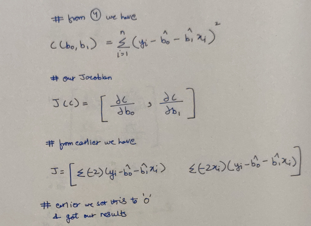 Our Jacobian
Well, if now, we can prove that determinant of our Hessian is positive (more strictly positive-definitive), then we can guarantee that at the expressions (Eq 5 & 8) we found earlier, we have achieved our Minima.
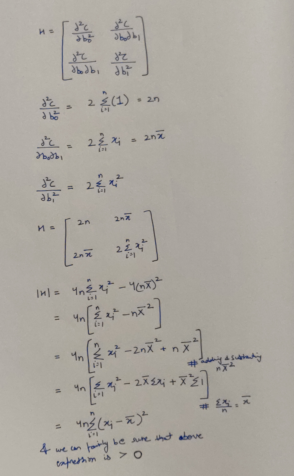 Concluding evidence from the Hessian
Our expression above, could also have the value 0, which will invalidate our conclusion of Minima, however that case will only arise when all x_i are some same constant. And this case will violate the very first assumption we made in the top! Hence we can safely ignore this and rejoice that we are correct.
We now atleast are at the level, from where we can touch the feet of Lord Vishnu. Hope I was able to help you out with the concepts mentioned! If not please leave feedback in comments as to how I can improve, since I plan to continue the Know The Math series. Am also attaching some references for additional information.
References
- http://seismo.berkeley.edu/~kirchner/eps_120/Toolkits/Toolkit_10.pdf
- https://www.mathsisfun.com/calculus/maxima-minima.html
- http://home.iitk.ac.in/~shalab/econometrics/Chapter2-Econometrics-SimpleLinearRegressionAnalysis.pdf
कर्मेन्द्रियाणि संयम्य य आस्ते मनसा स्मरन् ।
इन्द्रियार्थान्विमूढात्मा मिथ्याचारः स उच्यते ॥
– Bhagavad Gita 3.6 ॥
(Read about this Shloka from the Bhagavad Gita here at http://sanskritslokas.com/)
 NIFTYBANK - Time Series Analysis, Prediction & Hyper Parameter Optimization