DISCLAIMER - What this project is not:
- This project does not give any investment advice & is purely for research and academic purposes
- The analysis is based on data spanning 2 decades and the macro-economic scenario changes alone in that span, make it impractical for us to draw any inference in short term from this analysis
- The code is not meant for production, error-catching and logging mechanism have been skipped intentionally
AND IFF
- You like the project -> please star it on GitHub
- You find anything wrong -> please raise an issue in GitHub repository here
- You want to enhance/improve/help or contribute in any capacity -> please raise a PR in GitHub repository here
- You use any of the codes -> kindly provide a link back to this project or my profile on LinkedIn/GitHub (courtsey in Open Source) …there’s always scope in improving the code design!
I can’t recall ever once having seen the name of a market timer on Forbes’ annual list of the richest people in the world. If it were truly possible to predict corrections, you’d think somebody would have made billions by doing it.
- Peter Lynch
Hello reader, this project is completetly about Time Series - its analysis, prediction modelling and hyperparameter optimization(HPO) - specifically Bayesian HPO using Gausian Processes. I have made sure that the code is reusable. You can find some cool coding hacks and extensive API usage of libraries in the code. What’s more?! Since the code is generic, you can also try it out on different data sets as well! We’ll employ ARIMA, Deep Learning - CNNs, LSTMs & the likes. It’s going to be extremely technical, all code has been open sourced here and I have tried my best to aid you with explicit code comments and annotations. The project has been implemented in Python & following are the libraries utilised:
- Deep Learning library - tf.keras (yes, there’s difference between this and Keras)
- Visualization library - Bokeh
- Hyperparameter Optimization library - Skopt (scikit-optimize)
- Data processing library - Pandas, Numpy, sklearn & statsmodels
Will also be writing in detail in upcoming weeks about underlying math and theory of the concepts involved in the project!
I attended CFA Society, India’s webinar on 11th April ‘20 by Kriti Mahajan moderated by Shreenivas Kunte, CFA, CIPM on the topic- “Practitioners’ Insights: Using a Neural Network to Predict Stock Index Prices” which gave me the idea & inspiration to invest my time in this direction and this project was born!
P.S: Like always all code can be found here.
Objective
- To analyse a Time Series dataset (in this project - NIFTYBANK specifically, but you can use any dataset)
- To conduct Data exploration for understanding the data
- To process time-series data, normalise it and conduct data-stationarity testing
- To prepare benchmark in predictive modelling using traditional algorithms like ARIMA
- To apply Deep Learning techniques & try and improve on predictive modelling performance
- To automate modelling process
- To automate & apply Bayesian HPO techniques and find optimal hyperparameters for the models
- To automate & generate markdown document for each model which summarizes the model in its entirety - from architecture to HPO process to performance
Contents
- Data Exploration, Analysis & Processing
- Generating Benchmark using ARIMA
- Deep Neural Networks
- Navigating the Repo
- Acknowledgements
- References
Data Exploration, Analysis & Processing
The current index has 12 constituents of which Bandhan Bank was the newest entry (added when it went Public on 27th March 2018). Let’s see what the index looks like today (As of 19th June 2020)
| Company | Symbol | Sector | Ownership | Closing Price | Market Cap (Cr.) |
|---|---|---|---|---|---|
| Axis Bank | AXISBANK | Financial Services - Bank | Private | 417.05 | 117,691.88 |
| Bandhan Bank | BANDHANBNK | Financial Services - Bank | Private | 290.60 | 46,794.72 |
| Bank of Baroda | BANKBARODA | Financial Services - Bank | Public | 47.05 | 21,739.77 |
| Federal Bank | FEDERALBNK | Financial Services - Bank | Private | 50.95 | 10,156.17 |
| HDFC Bank | HDFCBANK | Financial Services - Bank | Private | 1,033.35 | 567,337.93 |
| ICICI Bank | ICICIBANK | Financial Services - Bank | Private | 363.80 | 235,585.60 |
| IDFC First Bank | IDFCFIRSTB | Financial Services - Bank | Private | 25.85 | 14,663.01 |
| IndusInd Bank | INDUSINDBK | Financial Services - Bank | Private | 483.65 | 33,544.02 |
| Kotak Mahindra | KOTAKBANK | Financial Services - Bank | Private | 1,302.50 | 257,739.27 |
| PNB | PNB | Financial Services - Bank | Public | 34.50 | 32,466.67 |
| RBL Bank | RBLBANK | Financial Services - Bank | Private | 168.90 | 8,592.13 |
| SBI | SBIN | Financial Services - Bank | Public | 184.50 | 164,659.08 |
For this project, I have worked on a private data set which has Time Series data comprising of more than 350 macro-economic variables pertaining to India. Currently I am trying to make it public so that everyone can explore it. The data spans 20 years starting from 2000-01-18 and ending at 2020-02-13.
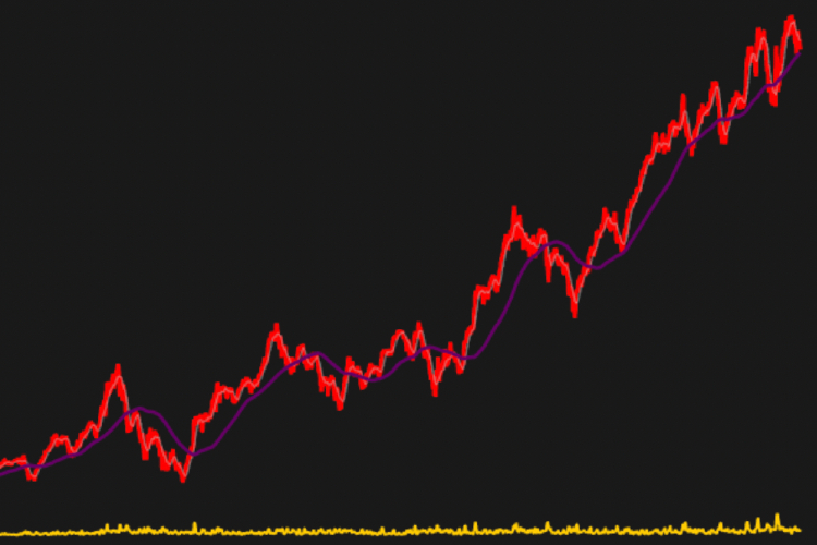
NIFTYBANK - A glance
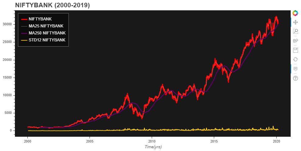 Nifty Bank progression over 2 decades based on closing prices
NIFTYBank has come a long way since it’s inception. At first look, it’s quite difficult to judge for variance for this data. However, just by looking at mean progression: one can conclude that this data is not covariance stationary.
Checking for Covariance Stationarity
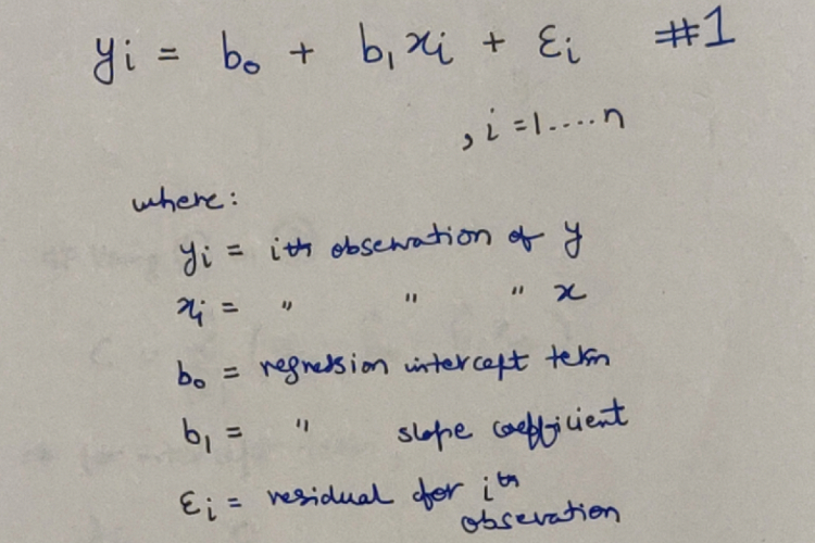
Time series modelling is quite challenging. We need to mathematically check for covariance stationarity on our data and if not, we need to transform the data such that it becomes stationary. Let’s check for the same on our data. We’ll use the Augmented Dickey-Fuller statistical test for this. Here’s a snippet that’ll give you an idea on how we can conduct this test:
  import pandas as pd
  from statsmodels.tsa.stattools import adfuller as aft

  def apply_aft_test_to_df_column(df_column: 'DataFrame column') -> dict:
      """Applies AFT Stationarity checking test to given DataFrame Column & returns calculated parameters as dict."""

      # Conduct AFT test on the given DF Column
      t_stat,p_val,no_of_lags,no_of_observation,crit_val,_ = aft(df_column, autolag='AIC')

      return {'T Stat':t_stat,'P value':p_val,'Number of Lags':no_of_lags,'Number of Observations':no_of_observation,'Critical value @ 1%':crit_val['1%'],'Critical value @ 5%':crit_val['5%'],'Critical value @ 10%':crit_val['10%']}

  # df = OUR DATA THAT WE WANT TO CHECK FOR COVARIANCE STATIONARITY
  df_columns = df.columns.values
  data_stationarity_information = {}

  for column in df_columns:
      # Conducting AFT test for specific column
      response = DataStationarityUtils.apply_aft_test_to_df_column(df[column])
      # Storing AFT test results for the column
      data_stationarity_information[column] = response

  # Converting stored AFT results into DataFrame
  data_stationarity_information_df = pd.DataFrame.from_dict(data_stationarity_information, orient='index')
  data_stationarity_information_df.index.name = "Features"
  # Generating stationarity verdict
  data_stationarity_information_df['Stationarity Verdict'] = data_stationarity_information_df['P value'] < 0.05
Here are the results:
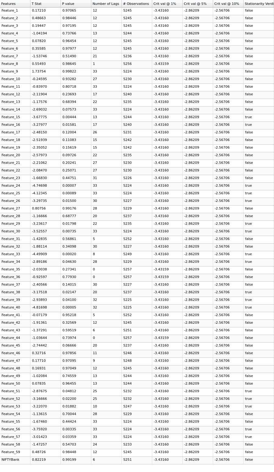 ADF Test results & verdict on stationarity over all features in dataset
Quite a few features are not stationary, especially our dependent feature of NIFTYBank. We could have gone ahead with the same data for our modelling as all features are cointegrated (economically linked to same macro-economic variables), but presence of few stationary features pose a problem. Hence, we’ll make all features stationary by transforming the data for daily returns of all the features, and then checking for stationarity. Here is how we can transform our data:
  # Assuming df = our DATA which we want to transform
  df_columns = df.columns.values
  daily_pct_change_df = pd.DataFrame(index=df.index)

  # Generating new columns as percentage change
  # on a single day basis
  for col in df_columns:
      daily_pct_change_df[f'{col} returns'] = df[col].pct_change(1)

  # Dropping first row as it contains all NAN values!
  daily_pct_change_df.drop(daily_pct_change_df.index[0],inplace=True)
Here is a glance at NIFTYBank Returns:
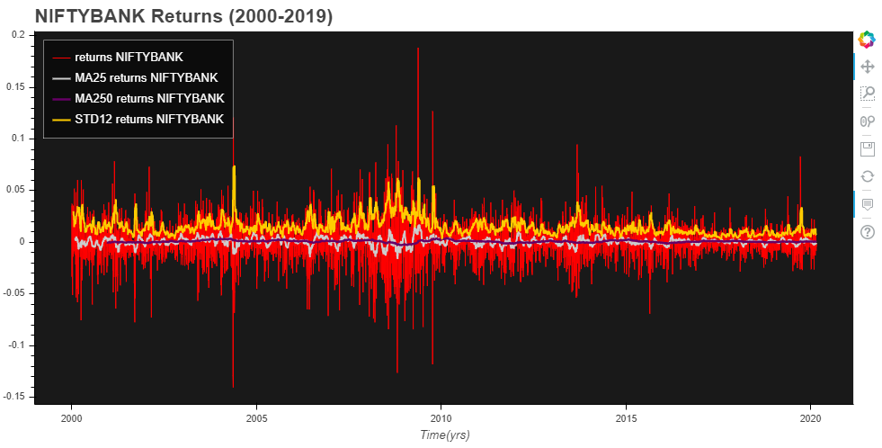 Nifty Bank Returns progression over 2 decades based on closing prices
Let’s check for covariance stationarity on this transformed data (All calculated P-values are very small, close to zero & have been rounded off to 5 decimal places in the below result):
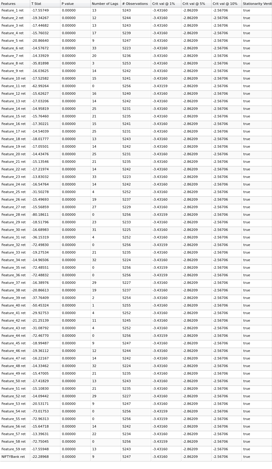 ADF Test results & verdict on stationarity over all features in transformed dataset
We can now safely conclude that the dataset can be called covariance stationary and proceed with further processing.
Normalizing the Data
We know that our features have different ranges and even follow their own different distributions, and this can cause issues when we use this data in our models. An easily observable issue is that some features might influence the result more/less than others. We will first standardize our data by calculating Z-score for every data point across all features. This will ensure that our data has a mean tending to zero and standard deviation tending to 1. And then, we’ll apply feature scaling to range [-1,1] to ensure that all features abide by these ranges.
  # Assuming we have split our data into training, validation & testing sets
  # (Refer to repository for splitting data util functions)
  # Here is how were are going to STANDARDIZE it:
  from sklearn.preprocessing import StandardScaler, MinMaxScaler

  normalizer = StandardScaler()
  # Remember we 'fit_transform' only on the TRAINING data
  standardized_training_data = normalizer.fit_transform(training_data.values)
  standardized_validation_data = normalizer.transform(validation_data.values)
  standardized_testing_data = normalizer.transform(testing_data.values)

  # The standardized data can now be fed for feature scaling
  minmax_scaler = MinMaxScaler(feature_range=(-1,1))
  minmax_norm_training_data = minmax_scaler.fit_transform(standardized_training_data)
  minmax_norm_validation_data = minmax_scaler.transform(standardized_validation_data)
  minmax_norm_testing_data = minmax_scaler.transform(standardized_testing_data)
Here is a visual aid to show effects of both these transformations on our data. (Have taken only the dependent variable here for illustration):
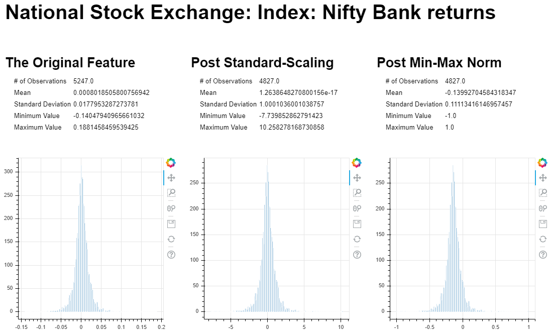 Effects of transformation on 1 of the features on our data
Do check the max and min values, mean and standard deviation across all plots above. It will definitely bring more clarity! Before proceeding further, let’s visit the constituents of NIFTYBANK briefly. (This analysis is part of my NIFTYBANK Portfolio Optimization & Efficient Frontier Generation project. You can visit the project’s repository here to get codes for this. Also, NIFTYBANK data from 4th April 2018 to 22th May 2020 has been considered for this.)
Correlation between all NIFTYBANK Index stocks
(Try it out here on this blog, it’s interactive!)
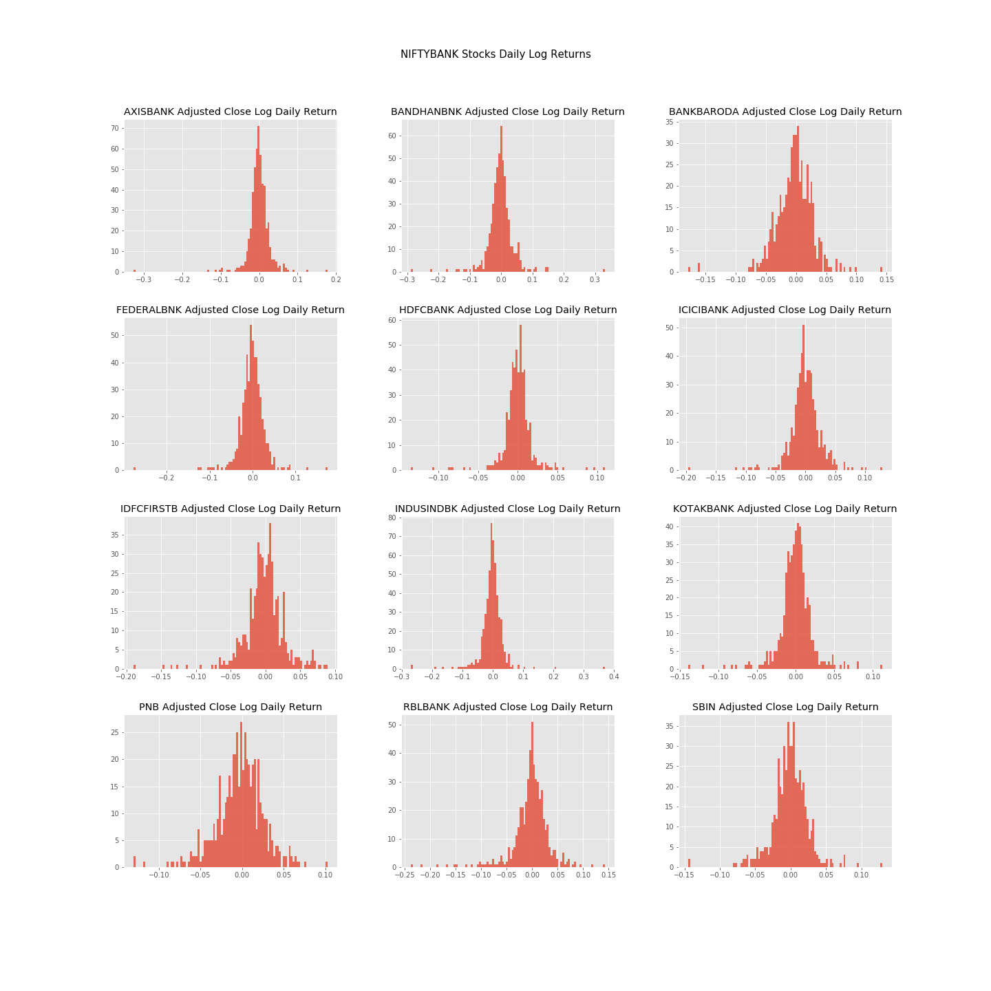
NIFTYBANK Index Stocks - Daily Lognormalized Returns
We can find out about the daily returns of all constituents by simply taking log of change of price at intervals of 1 day.
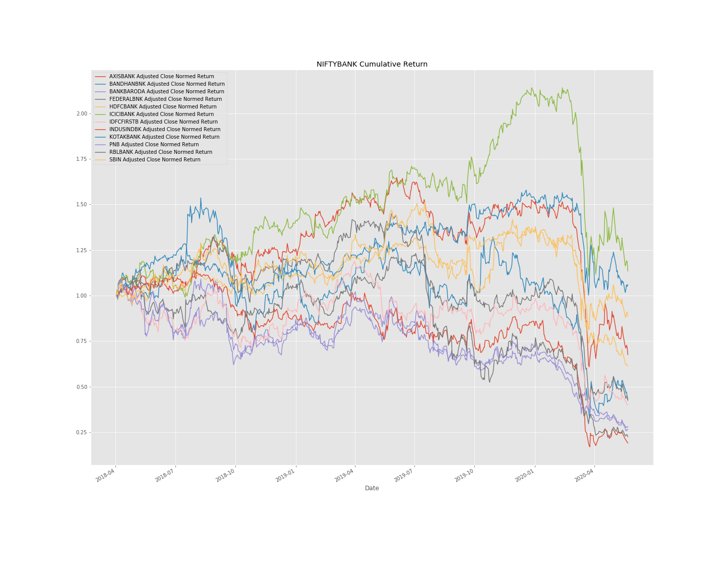
NIFTYBANK Index Stocks - Normalized Cumulative Returns
I have taken the base day as 4th April 2020, and calculated the cumulative returns with respect to that day.
Generating Benchmark using ARIMA
Let’s apply the widely known ARIMA model to our data. This is a traditional statistical algorithm, and we’ll consider results from this model as our benchmark for comparing other complex Deep Learning models. Let’s first have a look at Autocorrelation and Partial Autocorrelation function plots. Here is a snippet which will give us an idea on how we can do this:
  # Assuming df = DATA on which we wish to plot the ACF & PACF functions
  import statsmodels.graphics.tsaplots as tsaplots

  fig = plt.figure(figsize=(12,8))
  ax1 = fig.add_subplot(211)
  fig = tsaplots.plot_acf(df['Nifty Bank returns'].astype(float), lags=25, ax=ax1)
  ax2 = fig.add_subplot(212)
  fig = tsaplots.plot_pacf(df['Nifty Bank returns'].astype(float), lags=25, ax=ax2)
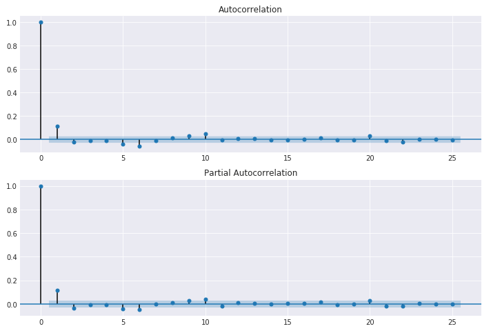 ACF & PACF Plots on our NIFTYBANK Returns dependent variable
A look at the plots tells us that with 95% confidence, correlation values post 1st lag are mostly statistical flukes and can safely be ignored i.e within 1st lag, AR is significant! This will help us decide on hyperparameters for our ARIMA model. These are the results I recieved:
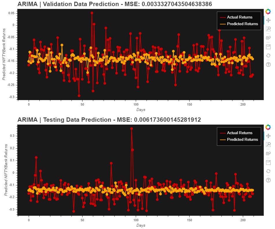 Prediction results & MSE on validation + test data via ARIMA model to be considered as a benchmark
Now that we somewhat have a benchmark, let’s try out Deep Neural Networks.
Deep Neural Networks
Let us now try and dive into Deep Neural Networks. I have prepared 2 very basic networks - a simple convolutional neural network and a simple LSTM network. Neural Networks are notoriously famous for their complex backend and black-box nature! I’ll be covering detailed analysis of these networks in upcoming weeks and add more complex models also. For now, you may refer the code in repository and try them out yourself! Here are some results from the auto-generated Markdown reports I achieved from these models.
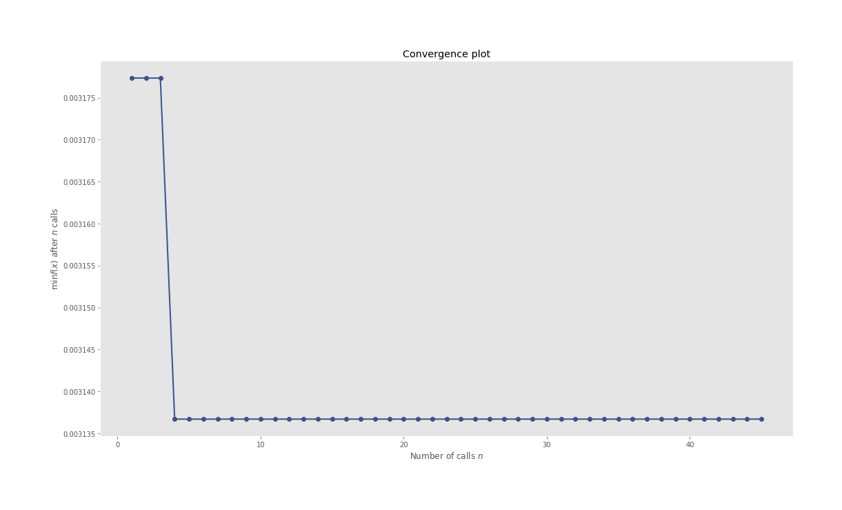
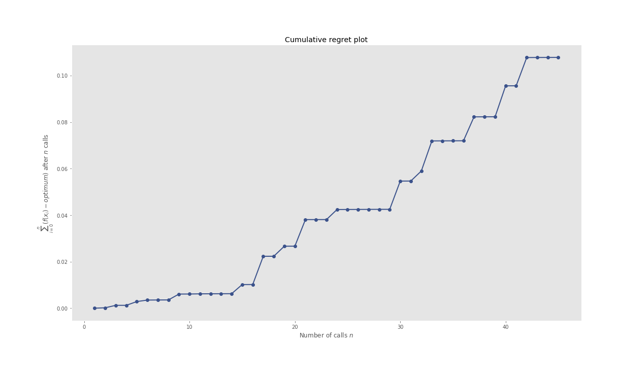
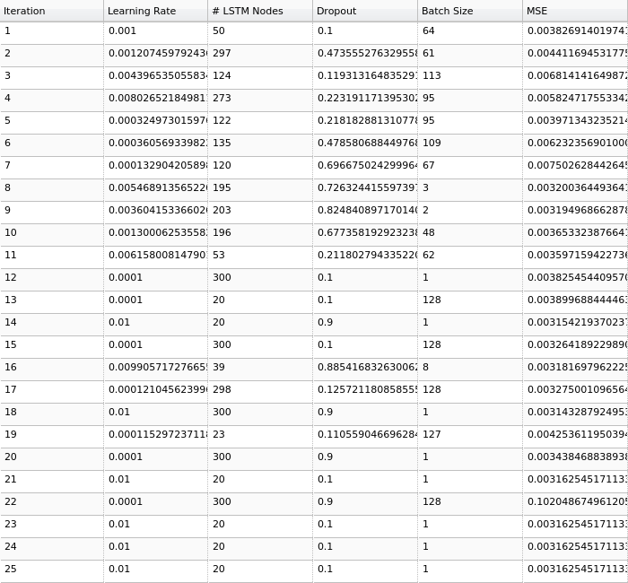
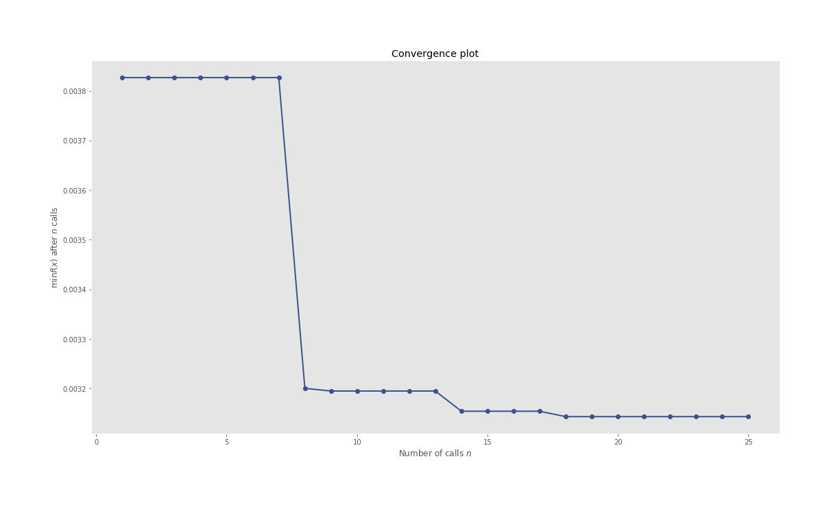
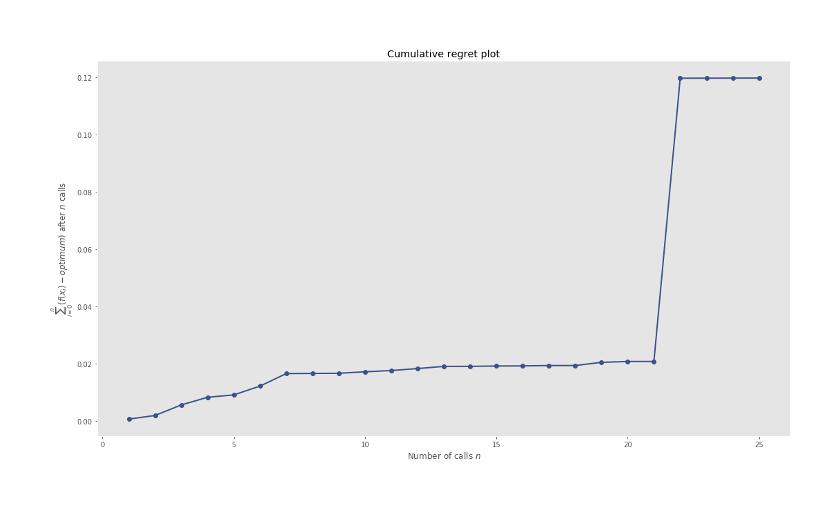
The ones which might catch your attention are HPO pertaining plots, especially the iterations plot where you can see what all candidate hyperparameters are considered sequentially by the BHPO method over the course of its iterations. Convergence plot shows us the progress of our optimization function in BHPO with the best result till the latest iteration.
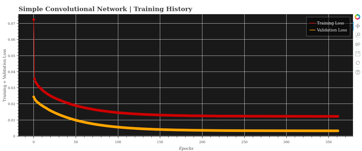
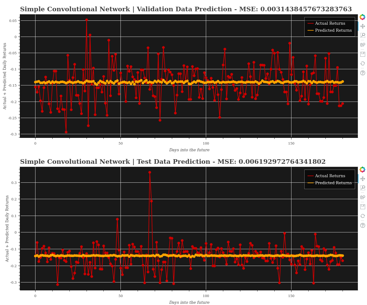
Above all, take the results with a pinch of salt. The data span of 2 decades can not be used to generate any inference over a short forecast period. (Interactive plots of the below graphs can be found in HTML files in this model’s assets in repository):
REPORTS
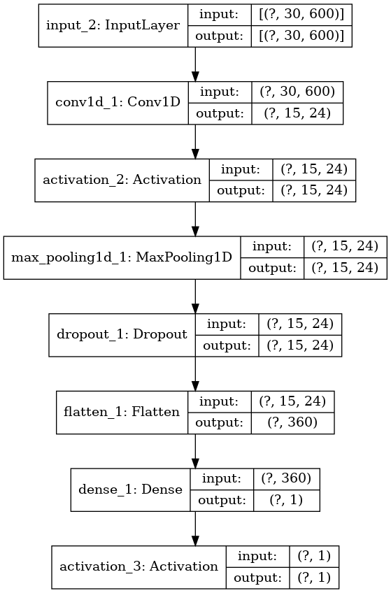
Simple Convolutional Neural Network
Model Summary
Model: "simple_convolutional_network"
_________________________________________________________________
Layer (type)                 Output Shape              Param #
=================================================================
input_2 (InputLayer)         [(None, 30, 600)]         0
_________________________________________________________________
conv1d_1 (Conv1D)            (None, 15, 24)            28824
_________________________________________________________________
activation_2 (Activation)    (None, 15, 24)            0
_________________________________________________________________
max_pooling1d_1 (MaxPooling1 (None, 15, 24)            0
_________________________________________________________________
dropout_1 (Dropout)          (None, 15, 24)            0
_________________________________________________________________
flatten_1 (Flatten)          (None, 360)               0
_________________________________________________________________
dense_1 (Dense)              (None, 1)                 361
_________________________________________________________________
activation_3 (Activation)    (None, 1)                 0
=================================================================
Total params: 29,185
Trainable params: 29,185
Non-trainable params: 0
Model Plot
Hyperparameter Optimization
Iterations & Results
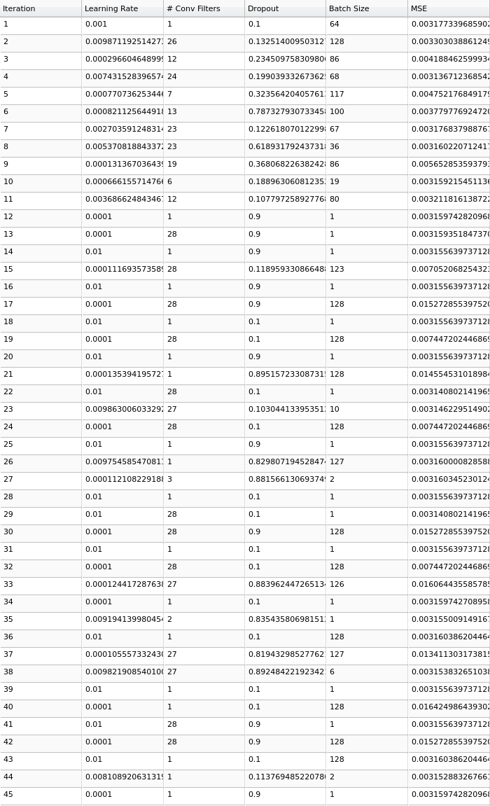
Convergence Plot
Evaluation Plot
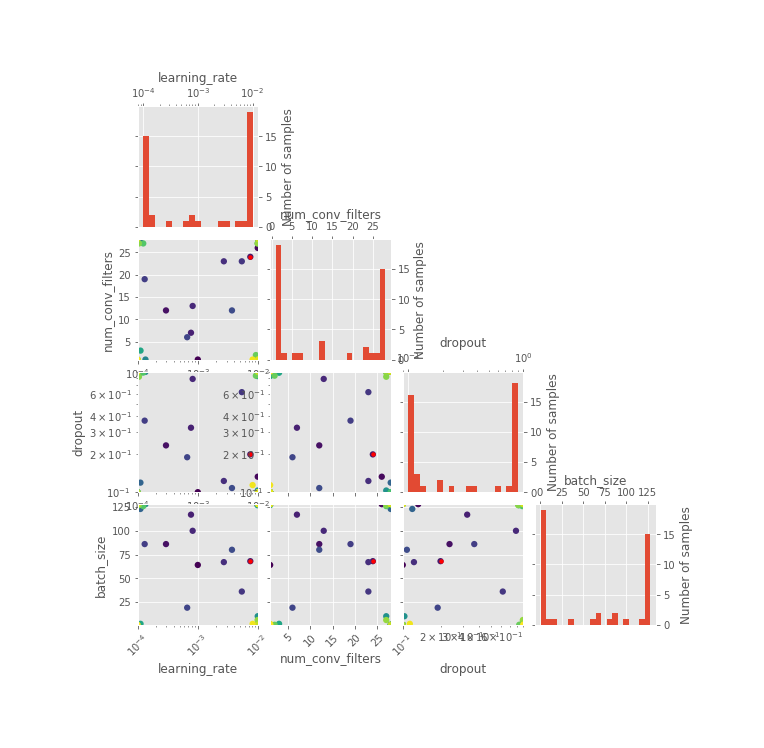
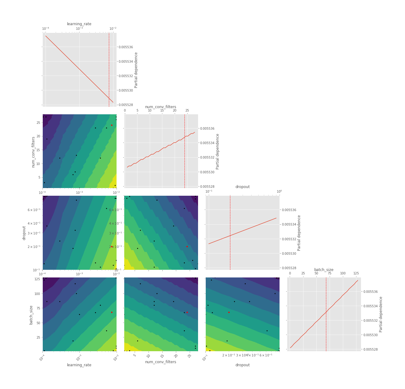
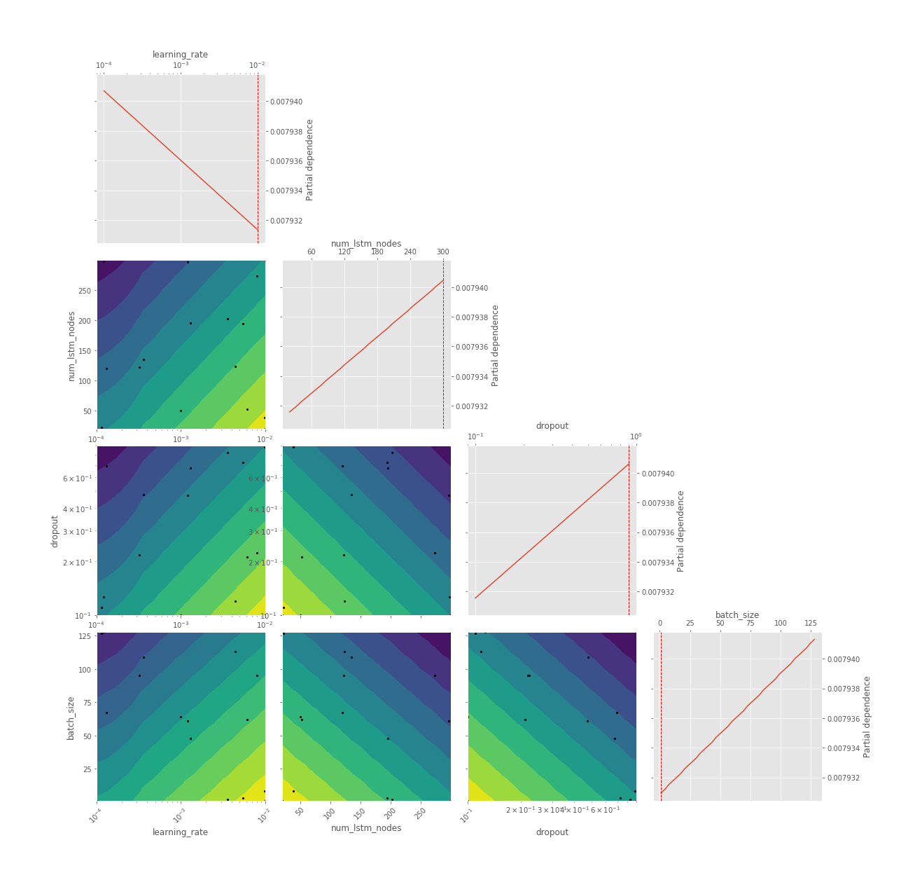
Objective Plot
Regret Plot
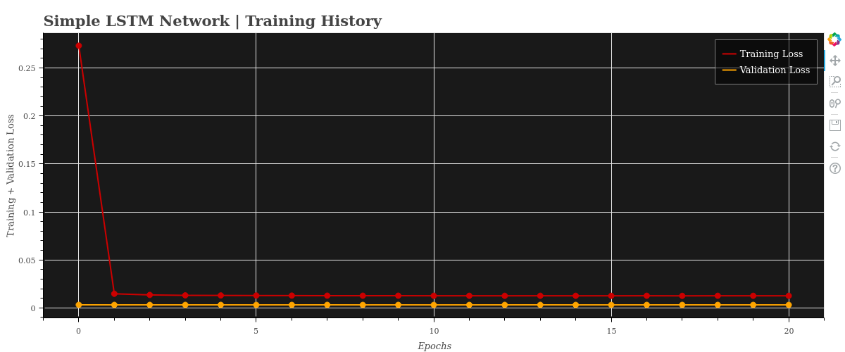
Model Training History
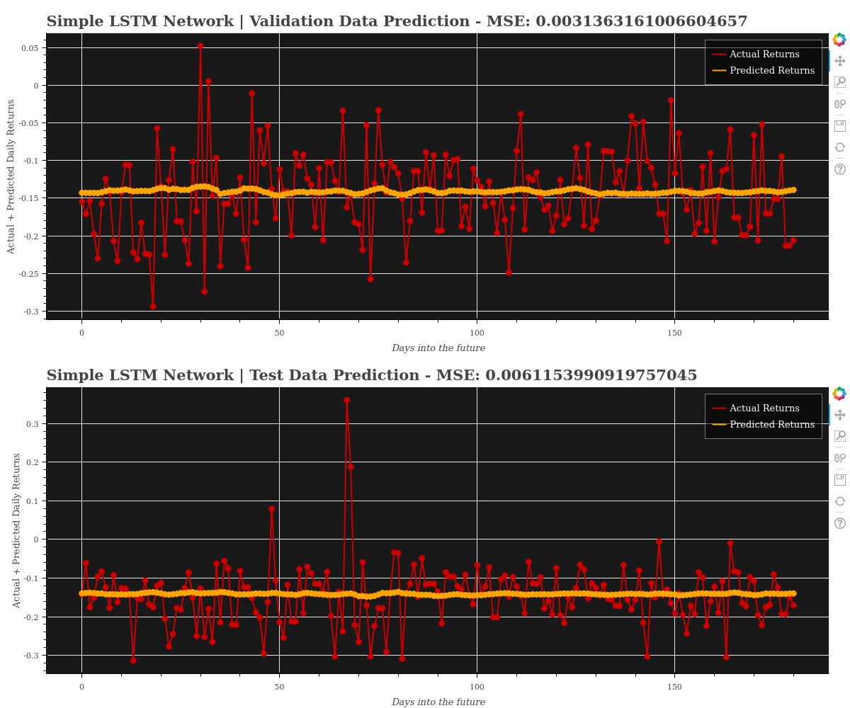
Model Predictions & MSE
Simple LSTM Network
Model Summary
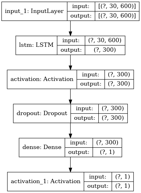
Model: "simple_lstm_network"
_________________________________________________________________
Layer (type)                 Output Shape              Param #
=================================================================
input_1 (InputLayer)         [(None, 30, 600)]         0
_________________________________________________________________
lstm (LSTM)                  (None, 300)               1081200
_________________________________________________________________
activation (Activation)      (None, 300)               0
_________________________________________________________________
dropout (Dropout)            (None, 300)               0
_________________________________________________________________
dense (Dense)                (None, 1)                 301
_________________________________________________________________
activation_1 (Activation)    (None, 1)                 0
=================================================================
Total params: 1,081,501
Trainable params: 1,081,501
Non-trainable params: 0
_________________________________________________________________
Model Plot
Hyperparameter Optimization
Iterations & Results
Convergence Plot
Evaluation Plot
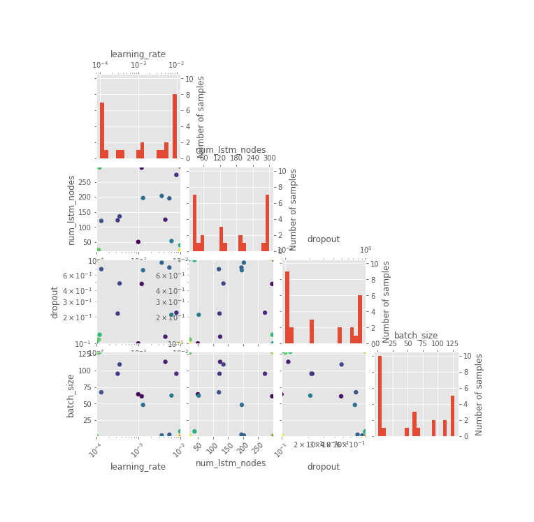
Objective Plot
Regret Plot
Model Training History
Model Predictions & MSE
Navigating the Repo
Here is quick primer to understand repository and structure of code:
.
├── assets
│   ├── simple_cnn
│   └── simple_lstm
├── config
│   └── model_configurations.py
├── initiate_predictive_modelling.py
├── LICENSE
├── models
│   └── neural_network_models.py
├── README.md
└── utils
    ├── data_processing_utils.py
    ├── data_stationarity_utils.py
    ├── data_visualization_utils.py
    └── model_utilities.py
- assets: You can find all plots, html files, markdown documents here
- config/model_configurations.py: You can find all config variables set here for the entire project
- initiate_predictive_modelling.py: A temporary piece of code I created over other utilities so that one can carry out end to end process and get a feel of things
- utils/data_processing_utils.py: You can find all Data processing tools here - reading CSV, dealing with NA, interpolation of data, saving df, computing lagged features, splitting time series data, data standardization, data normalization, etc
- utils/data_stationarity_utils.py: You can find functions here to check for covariance stationarity over given data
- utils/data_visualization_utils.py: You can find all visualization related functions here - bokeh utils, skopt plots, etc
- utils/model_utilities.py: You can find all model related utilities here - saving your model, generating predictions, conducting HPO, etc
- models/neural_network_models.py: Contains interfaces for all models that we prepare
If I’ve had your interest so far, let’s collaborate over GitHub and make this better. You can also reach out to me incase you have any queries pertaining to anything. Hope this helps!
Acknowledgements
My sincere thanks to Kriti Mahajan, Shreenivas Kunte, CFA, CIPM & CFA Society, India to conduct and host the webinar. It was quite insightful & gave me all the inspritaion I needed to take this project up. The entire session can be found here on Youtube.
References
Time Series modelling & tf.keras Resources
- Kriti Mahajan’s Colab Notebook https://colab.research.google.com/drive/1PYj_6Y8W275ficMkmZdjQBOY7P0T2B3g#scrollTo=mCTtyN5OP22z
- https://www.tensorflow.org/tutorials/structured_data/time_series
- https://www.tensorflow.org/api_docs/python/tf/keras
- https://www.tensorflow.org/guide/keras/sequential_model
- https://www.pyimagesearch.com/2019/10/28/3-ways-to-create-a-keras-model-with-tensorflow-2-0-sequential-functional-and-model-subclassing/
- https://www.pyimagesearch.com/2019/10/21/keras-vs-tf-keras-whats-the-difference-in-tensorflow-2-0/
Hyperparameter Optimization Resources
- https://www.kdnuggets.com/2018/12/keras-hyperparameter-tuning-google-colab-hyperas.html
- https://medium.com/@crawftv/parameter-hyperparameter-tuning-with-bayesian-optimization-7acf42d348e1
- https://github.com/Hvass-Labs/TensorFlow-Tutorials/blob/master/19_Hyper-Parameters.ipynb
- https://github.com/crawftv/Skopt-hyperparameter-tutorial/blob/master/scikit_optimize_tutorial.ipynb
- https://towardsdatascience.com/hyperparameter-optimization-in-python-part-1-scikit-optimize-754e485d24fe
- https://scikit-optimize.github.io/stable/
- https://www.kaggle.com/schlerp/tuning-hyper-parameters-with-scikit-optimize
- https://www.kdnuggets.com/2019/06/automate-hyperparameter-optimization.html
- https://towardsdatascience.com/hyperparameter-optimization-in-python-part-0-introduction-c4b66791614b
NIFTYBank Data Resources
- https://www.niftyindices.com/indices/equity/sectoral-indices/nifty-bank
- https://economictimes.indiatimes.com/markets/nifty-bank/indexsummary/indexid-1913,exchange-50.cms
- https://www.moneycontrol.com/stocks/marketstats/indexcomp.php?optex=NSE&opttopic=indexcomp&index=23
यदा यदा हि धर्मस्य ग्लानिर्भवति भारत।
अभ्युत्थानमधर्मस्य तदात्मानं सृजाम्यहम् ॥४-७॥परित्राणाय साधूनां विनाशाय च दुष्कृताम् ।
धर्मसंस्थापनार्थाय सम्भवामि युगे युगे ॥४-८॥
– Bhagavad Gita ॥
(Read about this Shloka from the Bhagavad Gita here at www.thedivineindia.com)
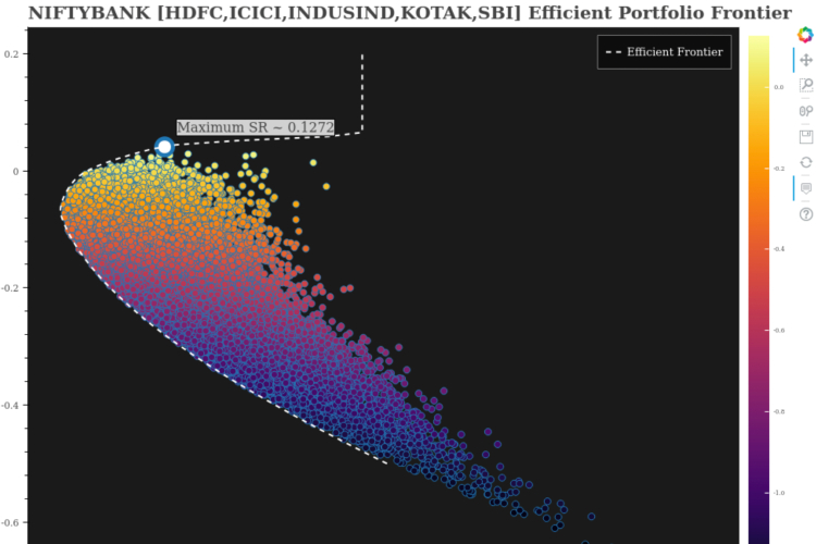 Portfolio Allocation & Efficient Frontier Generation