Portfolio Allocation & Efficient Frontier Generation

Hello reader, ever heard of the terms Asset/Portfolio allocation? If you have, chances are you’ve also heard about the MPT - Modern Portfolio Theory and Markovitz Efficient Frontier! Well this post and project are quite technical and will be based on these topics.

So sometime back, I finished the famous Python For Financial Analysis and Algorithmic Trading by the genius instructor Jose Portilla, on Udemy. In this project, I attempt to reuse the code provided in the course, extend it for generalization in Python and add some great interactive visualizations using Bokeh. I chose to work on NIFTYBANK Index Portfolio.

P.S: Like always all code can be found here on GitHub.

TL;DR - This is what this project attempts to achieve:

Objective

• Get some basic insights into the NIFTYBANK Index
• Conduct Monte Carlo Simulation over a portfolio to find the optimal mix of weights with maximum sharpe ratio possible
• Find and generate the efficient frontier for the portfolio
• All the above objectives have to be aided with crisp and interactive visualizations

Contents

1. Data Generation
2. Data Exploration
   1. Correlation between all NIFTYBANK Index stocks
   2. NIFTYBANK Index Stocks - Daily Lognormalized Returns
   3. NIFTYBANK Index Stocks - Normalized Cumulative Returns
3. Generating portfolios using Monte Carlo Simulation
4. Efficient Frontier Generation
5. Plotting the Efficient Frontier and Universe of Portfolios
6. Acknowledgements
7. References

Data Generation

Well, to work on a portfolio of NIFTYBANK we first need the data! The current index has 12 constituents of which Bandhan Bank was the newest entry(added when it went Public on 27th March 2018). Hence, for this project I have decided to work only on data from 4th April 2018 to 22th May 2020. Let’s see what the index looks like today (As of 25th May 2020)

Company	Symbol	Sector	Ownership	Closing Price	Market Cap (Cr.)
Axis Bank	AXISBANK	Financial Services - Bank	Private	341.30	96,313.68
Bandhan Bank	BANDHANBNK	Financial Services - Bank	Private	202.15	32,551.63
Bank of Baroda	BANKBARODA	Financial Services - Bank	Public	37.10	17,142.30
Federal Bank	FEDERALBNK	Financial Services - Bank	Private	38.45	7,663.49
HDFC Bank	HDFCBANK	Financial Services - Bank	Private	852.40	467,451.36
ICICI Bank	ICICIBANK	Financial Services - Bank	Private	292.70	189,517.39
IDFC First Bank	IDFCFIRSTB	Financial Services - Bank	Private	19.85	9,547.66
IndusInd Bank	INDUSINDBK	Financial Services - Bank	Private	348.20	24,149.75
Kotak Mahindra	KOTAKBANK	Financial Services - Bank	Private	1,153.20	220,699.92
PNB	PNB	Financial Services - Bank	Public	26.70	25,126.38
RBL Bank	RBLBANK	Financial Services - Bank	Private	110.55	5,623.80
SBI	SBIN	Financial Services - Bank	Public	151.40	135,118.62

Pandas_datareader + yfinance are going to be our best friends for getting Stock data free of charge on the run! This little code snippet should fix us up:

# Here are all our imports
import pandas_datareader.data as web
from pandas_datareader import data as pdr
import datetime
import pandas as pd
import yfinance as yf

# This is the magic line -> Essentially tells pandas_datareader to have Yahoo API backend engine
yf.pdr_override

# Giving time range for the data we need
start = datetime.datetime(2018, 4, 2)
end = datetime.datetime(2020, 5, 22)

# All constituents of NIFTYBANK Index
niftybank_stocks =['AXISBANK','BANDHANBNK','BANKBARODA','FEDERALBNK','HDFCBANK','ICICIBANK','IDFCFIRSTB','INDUSINDBK','KOTAKBANK','PNB','RBLBANK','SBIN']

# Creating our Data Frame object to store all stock data
index_col = pd.date_range(start=start, end=end)
nifty_bank_df = pd.DataFrame(index=index_col)
nifty_bank_df.index.name = 'Date'

# We iterate for all NIFTYBANK stocks, fetch their Adjusted Close
# Price from the API call and populate our data frame
for stock in niftybank_stocks:
    nifty_bank_df[f'{stock} Adjusted Close'] = pdr.get_data_yahoo(stock+'.NS', start, end)['Adj Close']

# Some basic cleaning required
# We have to remove all weekends!
nifty_bank_df = nifty_bank_df[(nifty_bank_df.index.dayofweek != 5)&(nifty_bank_df.index.dayofweek != 6)]

# And some other days which mostly are public holidays
# when Market is closed
nifty_bank_df = nifty_bank_df.dropna(axis=0,how='all')

# Finally we store our generated Data in CSV format
nifty_bank_df.to_csv('nifty_bank_df_2018-4-2_to_2020-5-22.csv',index_label='Date')

Data Exploration

Let’s try and churn out some insights from our generated data.

Correlation between all NIFTYBANK Index stocks

I have generated this correlation matrix using one of my other projects. You can find the entire code here in GitHub. (Try it out here on this blog, it’s interactive!)

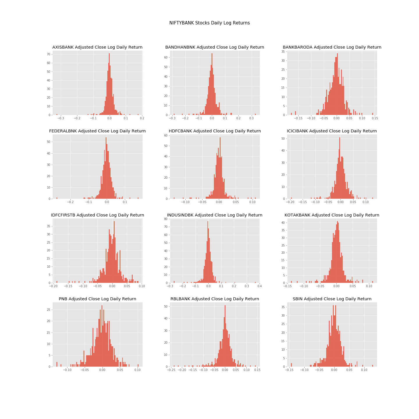
NIFTYBANK Index Stocks - Daily Lognormalized Returns

We can find out about the daily returns of all constituents by simply taking log of change of price at intervals of 1 day.

df_log_daily_return = pd.DataFrame(index=df.index)
df_log_daily_return.index.name = 'Date'
for column in df.columns.values:
    df_log_daily_return[f'{column} Log Daily Return'] = np.log(df[column]/df[column].shift(1))

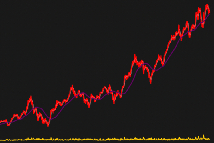
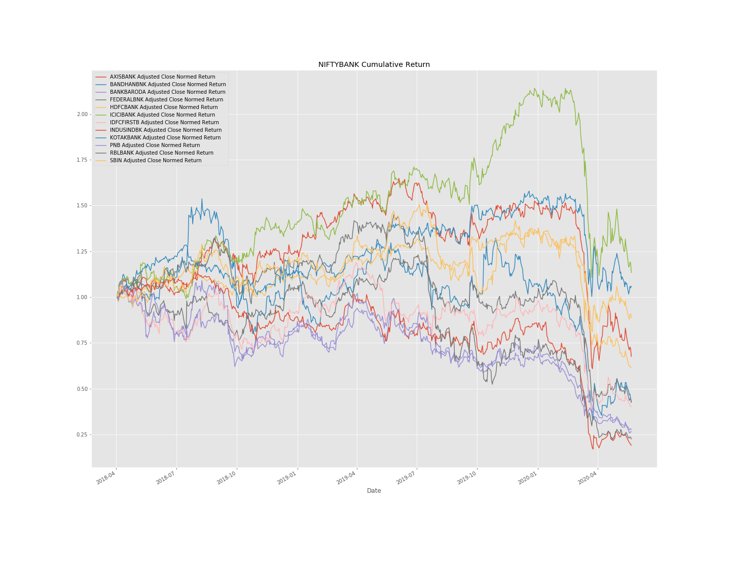
NIFTYBANK Index Stocks - Normalized Cumulative Returns

I have taken the base day as 4th April 2020, and calculated the cumulative returns with respect to that day.

df_normalised_return = pd.DataFrame(index=df.index)
df_normalised_return.index.name = 'Date'
for column in df.columns.values:
    df_normalised_return[f'{column} Normed Return'] = df[column]/df.iloc[0][column]

Generating portfolios using Monte Carlo Simulation

Well if you’ve reached till here - this is the fun part! We are going to create many - thousands of portfolios from our NIFTYBANK Index stocks. This is the basic idea - we have 12 stocks in our portfolio. We have to come up with as many portfolios as possible by allocating different weights to each these stocks. These weights we’ll be generating in a randomised manner over thousands of iterations. Imagine, each iteration will give us a new set of 12 random weights, each set of unique random weights will generate a new portfolio for us and each portfolio will have it’s own risk (volatility) and it’s return! Is there a fixed number of iterations or portfolios that we have to generate? No. There is not because there are infinitely many portfolios possible. However, generating a few thousand portfolios ought to give us some idea. Before we begin, some mythbusters:

1. “Portfolio with the maximum return is the best.” - NO
2. “Portfolio with the minimum risk is the best.” - NO
3. “Is there any correct answer to these questions?” - NO

In a nutshell, the answers are completely subjective and depend on the investor - her/his ability, willingness, appetite, etc. Let’s take this topic some other day!

Meanwhile let’s go through some Python which will help us with our portfolios:

• Input variable df is our previously created Data Frame which contains all our stock data

def generate_all_portfolios(df: 'Data Frame of all stocks', returns_mean: 'Mean Data Frame of all Stocks', returns_covariance: 'Covariance Data Frame of all stocks', number_of_portfolios: 'int' = 5000) -> 'dict':
    """Runs Monte Carlo simulation and creates desired number of portfolios for universe. Taken from Jose's abovementioned course!"""
    
    # Seeting seed for future reproducibility
    np.random.seed(55)

    number_of_stocks = len(df.columns)

    # Initializing portfolio particulars
    all_weights = np.zeros((number_of_portfolios,number_of_stocks))
    ret_arr = np.zeros(number_of_portfolios)
    vol_arr = np.zeros(number_of_portfolios)
    sharpe_arr = np.zeros(number_of_portfolios)

    # Beginning our iterations and generating all the portfolios
    for index in tqdm(range(number_of_portfolios)):

        # Here we generate the random weights for our stocks
        weights = np.array(np.random.random(number_of_stocks))

        # We make sure that all weights lie between 0 and 1
        weights = weights / np.sum(weights)
        all_weights[index,:] = weights

        # We calculate annualised returns for our created portfolio
        # assuming 252 trading days in an year
        ret_arr[index] = np.sum(returns_mean * weights *252)

        # We calculate the annualised volatility (standard deviation)
        # for our portfolio by exploiting some wicked Linear Algebra
        vol_arr[index] = np.sqrt(np.dot(weights.T, np.dot(returns_covariance * 252, weights)))

        # Finally we find out the Sharpe Ratio for our portfolio
        # assuming 0 (Zero) Risk Free rate
        sharpe_arr[index] = ret_arr[index]/vol_arr[index]
    
    return {
        'max_sharpe_ratio': sharpe_arr.max(),
        'max_sharpe_ratio_index': sharpe_arr.argmax(),
        'max_sharpe_ratio_return': ret_arr[sharpe_arr.argmax()],
        'max_sharpe_ratio_volatility': vol_arr[sharpe_arr.argmax()],
        'all_portfolio_weights': all_weights,
        'all_portfolio_returns': ret_arr,
        'all_portfolio_volatility': vol_arr,
        'all_portfolio_sharpe_ratio': sharpe_arr
    }

Efficient Frontier Generation

Efficient Frontier in layman terms is the set of portfolios wherein we get set of portfolios with maximum return for any given risk, or lowest risk for any given return. And therefore, anyone opting for portfolio which lies inside the efficient frontier is essentially just taking on more risk which will not be rewarded with extra return i.e. sub-optimal portfolio! We’ll be relying heavily on the Scipy mathematical computation Python library for achieving this.

• Inputs frontier_min_return and frontier_max_return to the below function are simply the range of returns over which we wish to find optimal portfolios

from scipy.optimize import minimize

def generate_efficient_frontier(number_of_stocks: 'int', frontier_min_return: 'float', frontier_max_return: 'float', number_of_frontier_portfolios: 'int' = 100) -> 'Frontier Volatility & Returns, lists':
    """Generates efficient frontier for the given range of desirable portfolio returns. Taken from Jose's abovementioned course!"""
    
    frontier_volatility = []

    # We generate 'number_of_frontier_portfolios' number of returns between our return ranges
    # so that we can generate optimal portfolios amongst them!
    frontier_returns = np.linspace(frontier_min_return, frontier_max_return, number_of_frontier_portfolios)

    # Initial weights that we choose for our portfolio
    init_guess = [1/number_of_stocks]*number_of_stocks

    # Contraining the bounds for each weight between 0 & 1
    bounds = tuple([(0,1) for _ in range(number_of_stocks)])

    # Iterating over different returns and churning out
    # portfolios with minimum risk
    for possible_return in tqdm(frontier_returns):
        cons = ({'type':'eq','fun': PortfolioGenerator.check_sum},
                {'type':'eq','fun': lambda w: get_ret_vol_sr(w)[0] - possible_return}
            )
        
        # GROUND ZERO - the real magic of SCIPY-optimize happens here
        result = minimize(minimize_volatility,init_guess,method='SLSQP',bounds=bounds,constraints=cons)
        
        # Storing the volatility of the generated portfolio
        frontier_volatility.append(result['fun'])

    return frontier_volatility, frontier_returns

Plotting the Efficient Frontier and Universe of Portfolios

And now at last, we have to visualise our universe of created portfolios and efficient frontier mentioned in above sections. I have deliberatly not embedded interactive versions of the plots here as they were making the site pretty heavy. You can head over to the repository and checkout all the Plot HTML files and play around with them.

def plot_efficient_frontier(title: 'str', plot_save_path: 'str', plot_image_save_path: 'str', all_portfolio_volatility: 'np array', all_portfolio_returns: 'np array', all_portfolio_sharpe_ratio: 'np array', max_sharpe_ratio_location: '[x,y] Coordinates', max_sharpe_ratio: 'float', efficient_frontier_returns: 'list', efficient_frontier_volatility: 'list', plot_width: 'int' = 1000, plot_height: 'int' = 800, axes_labels: '[X-axis label, Y-axis label]' = ['Portfolio Volatility', 'Portfolio Returns']) -> 'Bokeh Plot Object':
    """Generates plot for the entire portfolio universe and efficient frontier curve."""

    # Creating a color mapper so that we have a smooth gradient type color 
    # effect for portfolios ranging from lowest to highest Sharpe Ratio
    mapper = LinearColorMapper(palette=inferno(256), low=all_portfolio_sharpe_ratio.min(), high=all_portfolio_sharpe_ratio.max())

    # Preparing main ColumnDataSource which will be fed to the Bokeh Plot
    source = ColumnDataSource(data=dict(all_portfolio_volatility = all_portfolio_volatility, all_portfolio_returns = all_portfolio_returns, all_portfolio_sharpe_ratio = all_portfolio_sharpe_ratio))

    # Initializing our Bokeh Plot
    p = figure(plot_width=plot_width, plot_height=plot_height, toolbar_location='right', x_axis_label=axes_labels[0], y_axis_label=axes_labels[1], tooltips=[('Sharpe Ratio', '@all_portfolio_sharpe_ratio'),('Portfolio Return', '@all_portfolio_returns'),('Portfolio Volatility', '@all_portfolio_volatility')])

    # Adding circular rings for Sharpe Ratios of each portfolio
    p.circle(x='all_portfolio_volatility', y='all_portfolio_returns', source=source, fill_color={'field': 'all_portfolio_sharpe_ratio', 'transform': mapper}, size=8)

    # Adding circular ring for Maximum Sharpe Ratio portfolio
    p.circle(x=max_sharpe_ratio_location[0], y=max_sharpe_ratio_location[1], fill_color='white', line_width=5, size=20)

    # Adding Text annotation for Maximum Sharpe Ratio portfolio
    maximum_sharpe_ratio_portfolio = Label(x=max_sharpe_ratio_location[0]+0.005, y=max_sharpe_ratio_location[1]+0.02, text=f'Maximum SR ~ {round(max_sharpe_ratio, 4)}', render_mode='css', border_line_color='black', border_line_alpha=1.0, background_fill_color='white', background_fill_alpha=0.8)
    p.add_layout(maximum_sharpe_ratio_portfolio)

    # Adding the Efficient Frontier curve to our plot
    p.line(x=efficient_frontier_volatility, y=efficient_frontier_returns, line_width=2, line_color='white', legend='Efficient Frontier', line_dash='dashed')

    # Adding a color bar to indicate about varying Sharpe Ratio
    color_bar = ColorBar(color_mapper=mapper, major_label_text_font_size="5pt",ticker=BasicTicker(desired_num_ticks=10),formatter=PrintfTickFormatter(format="%.1f"),label_standoff=6, border_line_color=None, location=(0, 0))
    p.add_layout(color_bar, 'right')

    # Adding title to our plot
    p.add_layout(Title(text=title, text_font_size="16pt"), 'above')
    p.title.text_font_size = '20pt'

    # Fixing up Plot properties
    p.background_fill_color = "black"
    p.background_fill_alpha = 0.9
    p.xgrid.grid_line_color = None
    p.ygrid.grid_line_color = None

    # Fixing up Plot legend
    p.legend.background_fill_alpha = 0.5
    p.legend.background_fill_color = 'black'
    p.legend.label_text_color = 'white'
    p.legend.click_policy = 'mute'

    # Saving the plot
    output_file(plot_save_path)
    save(p)
    export_png(p, filename = plot_image_save_path)

    return p

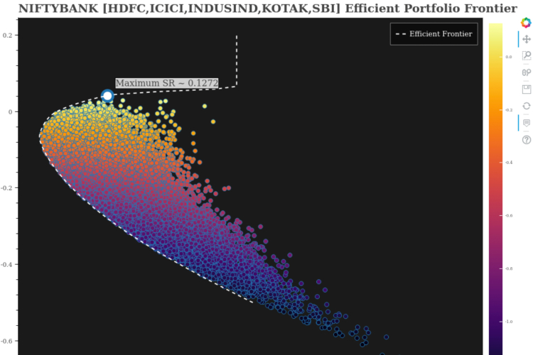
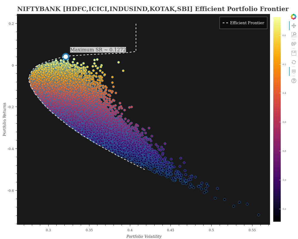
NIFTYBANK - HDFC,ICICI,INDUSIND,KOTAK,SBI - Efficient Portfolio Frontier

Owing to hardware limitation from my end, I first tried with only the abovementioned constituents of NIFTYBANK. Here is what the plot looks like:

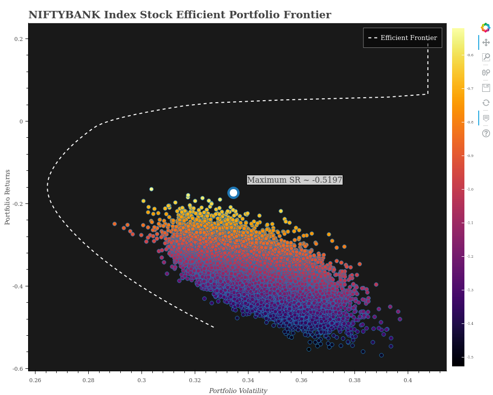
However, am also adding what I came up with for the entire NIFTBANK portfolio universe. Please note this is misleading. Reasons:

• Since the universe of 12 constituents is too big, we need several hundreds of thousands of iterations to even begin to get an idea about the universe. However, my hardware limitations allowed me only a few thousand portfolios which you see in the Plot.
• Nevertheless, the efficient frontier does give us some sort of an idea about our portfolio universe and what our possible optimal set of portfolios could have been
• The max Sharpe Ratio pointed out on this one, is only for the portfolios that we have generated from our limited number of iterations!

This was basically the entire project. If you’re up for it, let’s collaborate over GitHub and make this better. You can also reach out to me incase you have any queries pertaining to Bokeh or anything Python. Hope this helps!

Acknowledgements

My sincere thanks to Jose Portilla and Udemy for curating and delivering one of the best Financial Analysis courses ever!

References

• https://www.udemy.com/course/python-for-finance-and-trading-algorithms/
• https://www.niftyindices.com/indices/equity/sectoral-indices/nifty-bank
• https://economictimes.indiatimes.com/markets/nifty-bank/indexsummary/indexid-1913,exchange-50.cms
• https://www.moneycontrol.com/stocks/marketstats/indexcomp.php?optex=NSE&opttopic=indexcomp&index=23

कर्मण्येवाधिकारस्ते मा फलेषु कदाचन ।
मा कर्मफलहेतुर्भुर्मा ते संगोऽस्त्वकर्मणि ॥
                                                 – Bhagavad Gita ॥

(Read about this Shloka from the Bhagavad Gita here at www.pravakta.com)