Hello reader, welcome to my Know The Math series, a less formal series of blogs, where I take you through the notoriously complex backend mathematics which forms the soul for machine learning algorithms. The idea for the series originated from my Project - NIFTYBANK Index Time series analysis, Prediction, Deep Learning & Bayesian Hyperparameter Optimization where people also asked to explain the underlying concepts.
Before we begin, I need you to conduct a ceremony:
- Stand up in front of a mirror, and say it out aloud, “I am going to learn the Math behind Logistic Regression, today!”
- Take a out a naice register & pen to go through the derivation with me.
Before we begin, one surprise for the uninitiated - Logistic Regression is actually a classification algorithm. Let that sink in. Today, we are going to go through Binary Logistic Regression and the same concepts can be extended for multiclass problem.
Contents
- Getting The Idea
- Maximum Likelihood Estimation (MLE) & The Cost Function
- The Cost Function Gradient
- References
Getting The Idea
Well, since we have to classify our given input samples to 1 of the 2 classes, the clever way humans have found is to achieve this by finding probability for one of the classes (say Class 1). And if let’s say that, the found probability is greater than a chosen threshold (say >= 0.5), we can can conclude that it can be classified for 1st class; otherwise the 2nd one! The question now is, how do we find that magical probability? We start at the bottom -> from Linear Regression.
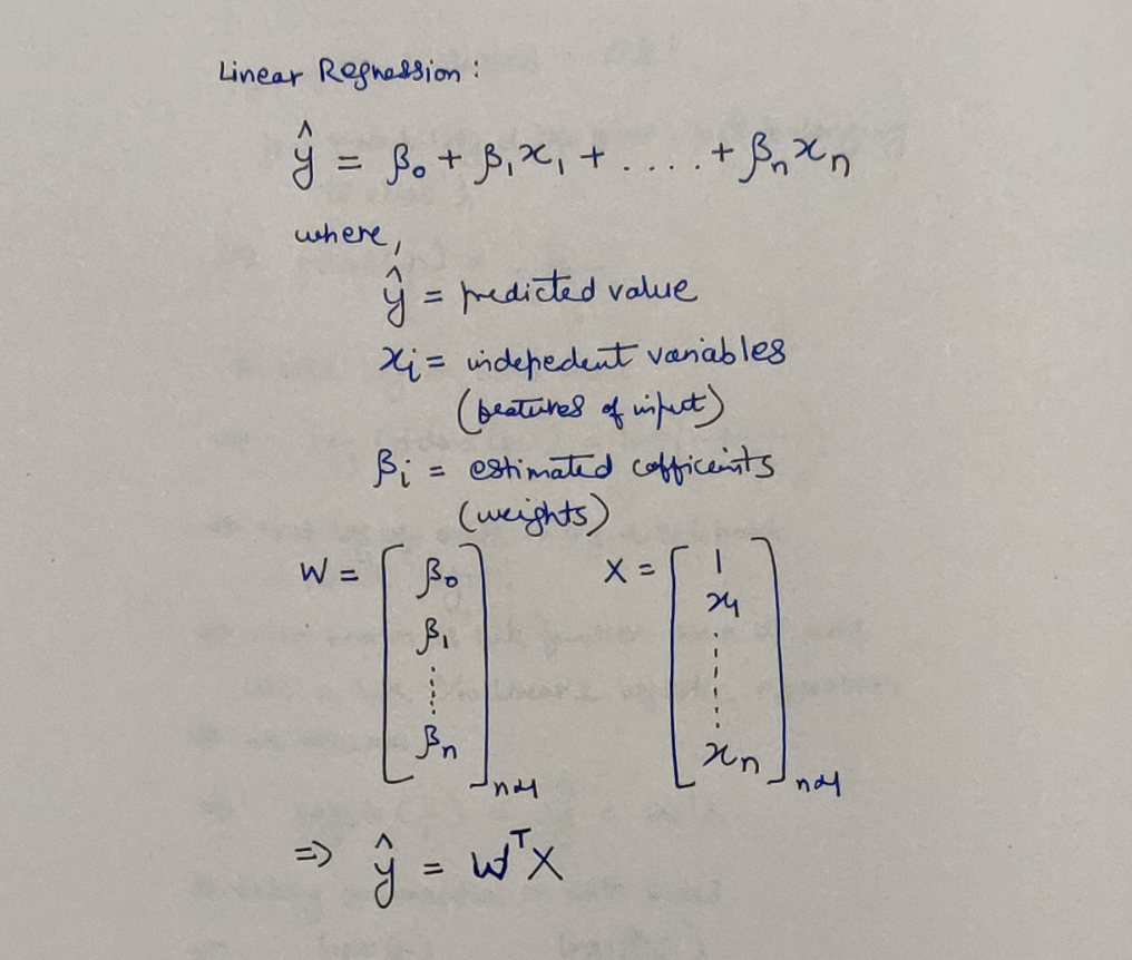 Linear Regression - The Unsung Hero
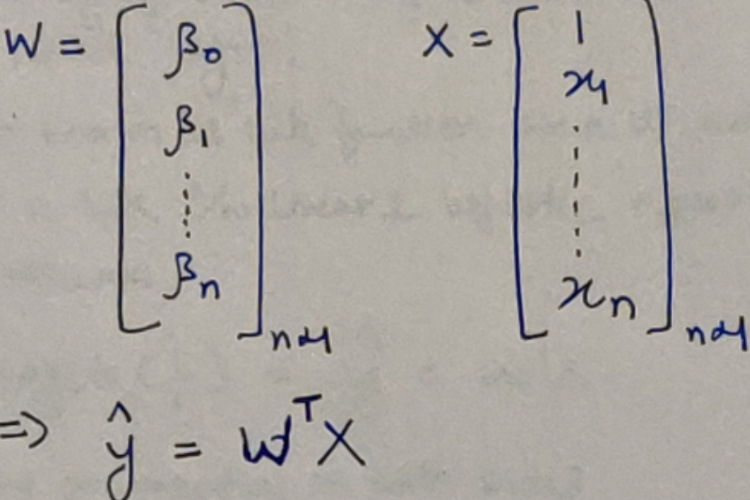
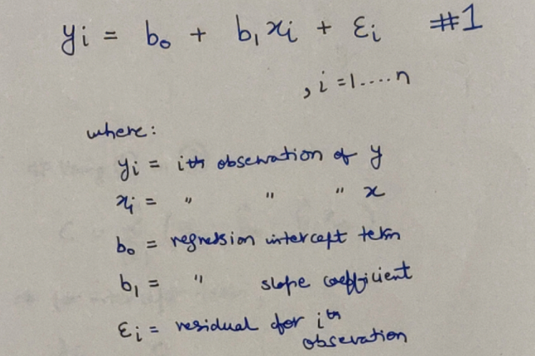
We can safely say, that the range of y is from negative infinity to positive infinity over the domain of x. We also know that probability of any event is bound by [0,1]. So is there anyway, by which we can make use of the above equation, apply some transformation to it and have the same bounds? Hear me out and solve with me:
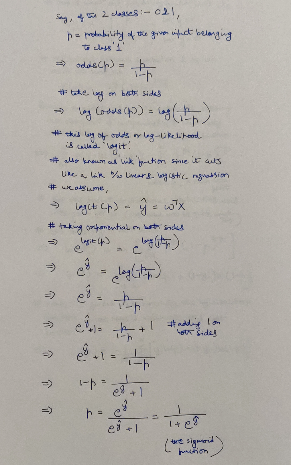 Logit & the Sigmoid
Maximum Likelihood Estimation (MLE) & The Cost Function
MLE is a statistical algorithm and is basically a probabilistic framework from estimating the parameters for a model. It’s vast potential leaves us with alot to appreciate and even more to understand, however, for our purpose we can continue like this:
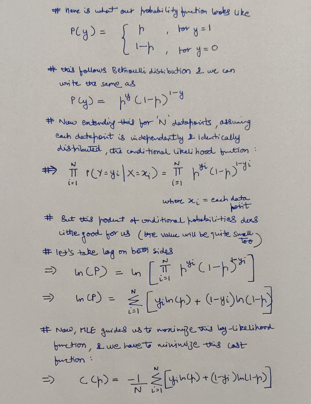 MLE and our Cost Function - The Cross Entropy
The Cost Function Gradient
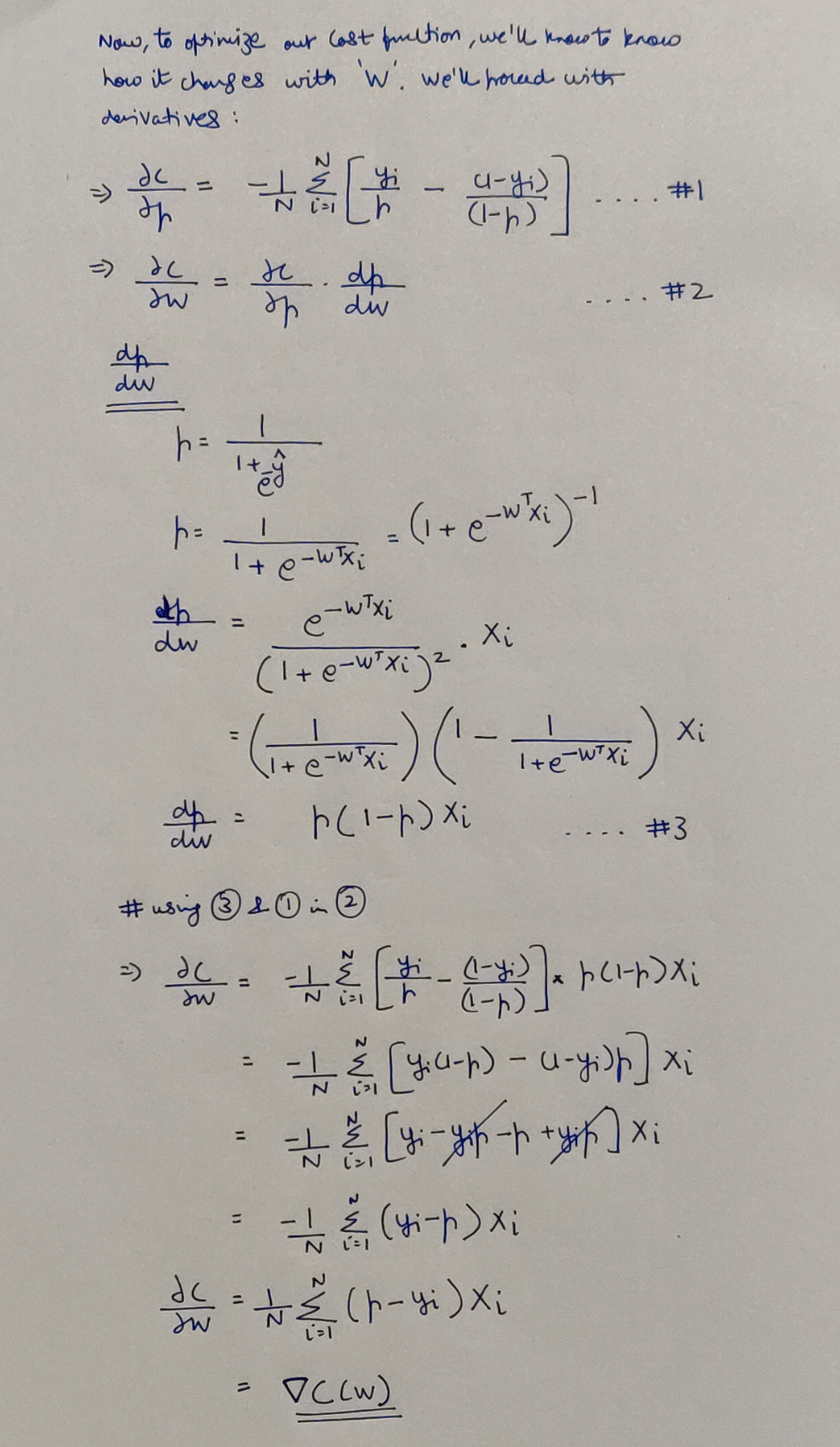 Finding the gradient of the cost function
From here on, we simply have to carry on the Gradient Descent algorithm which will iteratively update the W matrix by substracting the the above gradient times the chosen learning rate hyperparameter from the W matrix.
Hope I was able to help you out with the concepts mentioned! If not please leave feedback in comments as to how I can improve, since I plan to continue the Know The Math series. Am also attaching some references for additional information and sources which helped me write this blog.
References
- https://web.stanford.edu/class/archive/cs/cs109/cs109.1166/pdfs/40%20LogisticRegression.pdf
- https://towardsdatascience.com/an-introduction-to-logistic-regression-8136ad65da2e
- http://www.haija.org/derivation_logistic_regression.pdf
- https://machinelearningmastery.com/logistic-regression-with-maximum-likelihood-estimation/#:~:text=The%20parameters%20of%20a%20logistic,framework%20called%20maximum%20likelihood%20estimation.&text=The%20parameters%20of%20the%20model,Bernoulli%20distribution%20for%20each%20example.
- https://win-vector.com/2011/09/14/the-simpler-derivation-of-logistic-regression/
यो मामजमनादिं च वेत्ति लोकमहेश्वरम् ।
असम्मूढः स मर्त्येषु सर्वपापैः प्रमुच्यते ॥
– Bhagavad Gita 10.3 ॥
(Read about this Shloka from the Bhagavad Gita here at http://sanskritslokas.com/)
 Know The Math - Linear Regression & the Coefficients via Ordinary Least Squares